Engineering Economic Analysis Chapter 2 Engineering Costs and

Engineering Economic Analysis Chapter 2 Engineering Costs and Cost Estimating 3/16/2018 rd cw 2 a-1

Cost Explicit vs. Implicit Cash vs. Book Fixed vs. Variable Marginal vs. Average Sunk, Opportunity Recurring, Nonrecurring Incremental, Cash (out of pocket) vs. Book Life Cycle 3/16/2018 rd cw 2 a-2

Costs Life cycle First Operating & Maintenance Disposal Sunk Future Opportunity Direct Indirect Overhead Fixed Variable 3/16/2018 rd cw 2 a-33 cw 2 a-3

Cost Estimation What cost component must be estimated? What approach to cost estimation will be applied? How accurate should the estimates be? What estimation techniques will be utilized? 3/16/2018 rd cw 2 a-4

Cost Estimating What cost components must be estimated? First component ~ equipment, delivery, installation insurance, training Elements – Direct labor and materials, maintenance What approach to cost estimation will be applied? Bottom-up, design-to-cost or top-down How accurate should estimates be? ROMs ~ 20% of actual costs, Detail 5% What estimation techniques will be used? Unit, cost indices, learning curves, capacity, analogy 3/16/2018 rd cw 2 a-55 cw 2 a-5

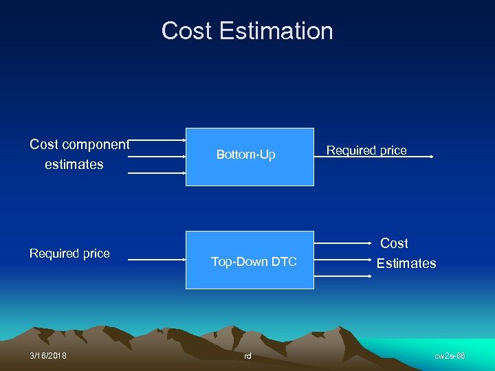Cost Estimation Cost component estimates Required price 3/16/2018 Bottom-Up Top-Down DTC rd Required price Cost Estimates cw 2 a-66 cw 2 a-6

First Component Equipment Cost Delivery charges Installation costs Insurance coverage Initial training of personnel for equipment use 3/16/2018 rd cw 2 a-7

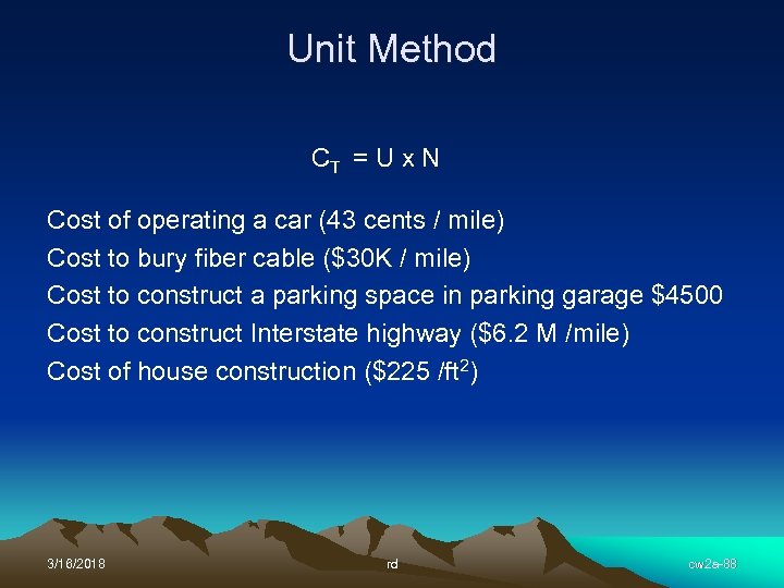Unit Method CT = U x N Cost of operating a car (43 cents / mile) Cost to bury fiber cable ($30 K / mile) Cost to construct a parking space in parking garage $4500 Cost to construct Interstate highway ($6. 2 M /mile) Cost of house construction ($225 /ft 2) 3/16/2018 rd cw 2 a-88 cw 2 a-8

Annual Operating Costs Direct labor cost for operating personnel Direct materials Maintenance (daily, periodic, repairs, etc. ) Rework and rebuild Can use canned cost estimating packages for bridges, pavement, etc. 3/16/2018 rd cw 2 a-9

Cost Estimates Rough Order of Estimates (ROMs) Semi-detailed Detailed (WBS) Segmented (divide and conquer) Analogy Parametric (e. g. , by foot or mile) Cost Index Triangulation (Delphi) Learning Curve 3/16/2018 rd cw 2 a-10

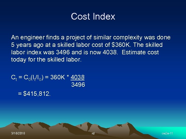Cost Index An engineer finds a project of similar complexity was done 5 years ago at a skilled labor cost of $360 K. The skilled labor index was 3496 and is now 4038. Estimate cost today for the skilled labor. Ct = C 0(It/I 0) = 360 K * 4038 3496 = $415, 812. 3/16/2018 rd cw 2 a-11

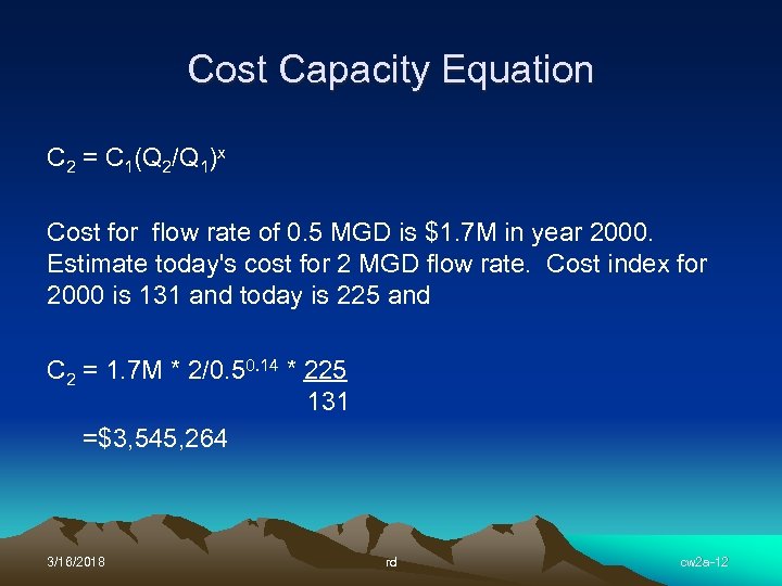Cost Capacity Equation C 2 = C 1(Q 2/Q 1)x Cost for flow rate of 0. 5 MGD is $1. 7 M in year 2000. Estimate today's cost for 2 MGD flow rate. Cost index for 2000 is 131 and today is 225 and C 2 = 1. 7 M * 2/0. 50. 14 * 225 131 =$3, 545, 264 3/16/2018 rd cw 2 a-12

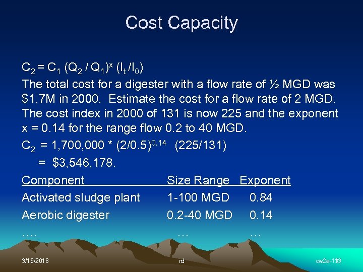Cost Capacity C 2 = C 1 (Q 2 / Q 1)x (It /I 0) The total cost for a digester with a flow rate of ½ MGD was $1. 7 M in 2000. Estimate the cost for a flow rate of 2 MGD. The cost index in 2000 of 131 is now 225 and the exponent x = 0. 14 for the range flow 0. 2 to 40 MGD. C 2 = 1, 700, 000 * (2/0. 5)0. 14 (225/131) = $3, 546, 178. Component Size Range Exponent Activated sludge plant 1 -100 MGD 0. 84 Aerobic digester 0. 2 -40 MGD 0. 14 …. … … 3/16/2018 rd cw 2 a-13 13 cw 2 a-13

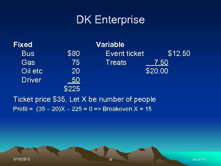DK Enterprise Fixed Bus Gas Oil etc Driver Variable Event ticket Treats $80 $12. 50 75 7. 50 20 $20. 00 50 $225 Ticket price $35, Let X be number of people Profit = (35 – 20)X – 225 = 0 => Breakeven X = 15 3/16/2018 rd cw 2 a-14

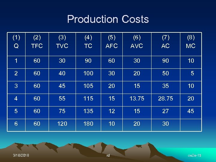Production Costs (1) Q (2) TFC (3) TVC (4) TC (5) AFC (6) AVC (7) AC (8) MC 1 60 30 90 10 2 60 40 100 30 20 50 5 3 60 45 105 20 15 35 10 4 60 55 115 15 13. 75 28. 75 20 5 60 75 135 12 15 27 45 6 60 120 180 10 20 30 3/16/2018 rd cw 2 a-15

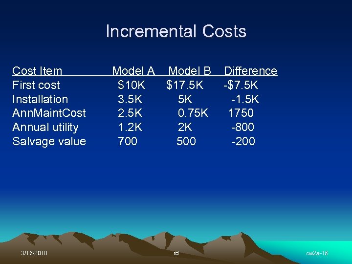Incremental Costs Cost Item First cost Installation Ann. Maint. Cost Annual utility Salvage value 3/16/2018 Model A Model B $10 K $17. 5 K 3. 5 K 5 K 2. 5 K 0. 75 K 1. 2 K 2 K 700 500 rd Difference -$7. 5 K -1. 5 K 1750 -800 -200 cw 2 a-16

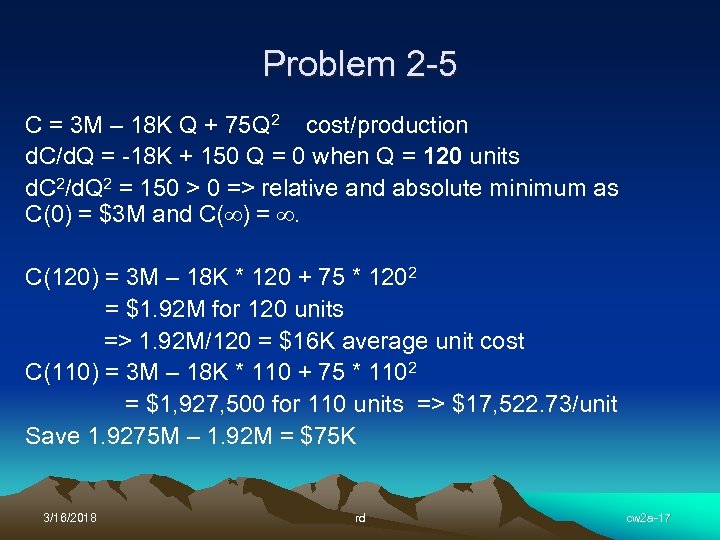Problem 2 -5 C = 3 M – 18 K Q + 75 Q 2 cost/production d. C/d. Q = -18 K + 150 Q = 0 when Q = 120 units d. C 2/d. Q 2 = 150 > 0 => relative and absolute minimum as C(0) = $3 M and C( ) = . C(120) = 3 M – 18 K * 120 + 75 * 1202 = $1. 92 M for 120 units => 1. 92 M/120 = $16 K average unit cost C(110) = 3 M – 18 K * 110 + 75 * 1102 = $1, 927, 500 for 110 units => $17, 522. 73/unit Save 1. 9275 M – 1. 92 M = $75 K 3/16/2018 rd cw 2 a-17

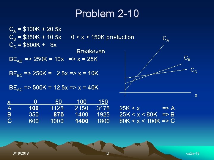Problem 2 -10 CA = $100 K + 20. 5 x CB = $350 K + 10. 5 x CC = $600 K + 8 x BEAB 0 < x < 150 K production CA Breakeven => 250 K = 10 x => x = 25 K CB CC BEBC => 250 K = 2. 5 x => x = 10 K BEAC => 500 K = 12. 5 x => x = 40 K x x A B C 0 100 350 600 3/16/2018 50 1125 875 1000 100 2150 1400 150 3175 1925 1800 rd 25 K < x => A 25 K < x < 80 K => B 80 K < x < 100 K => C cw 2 a-18

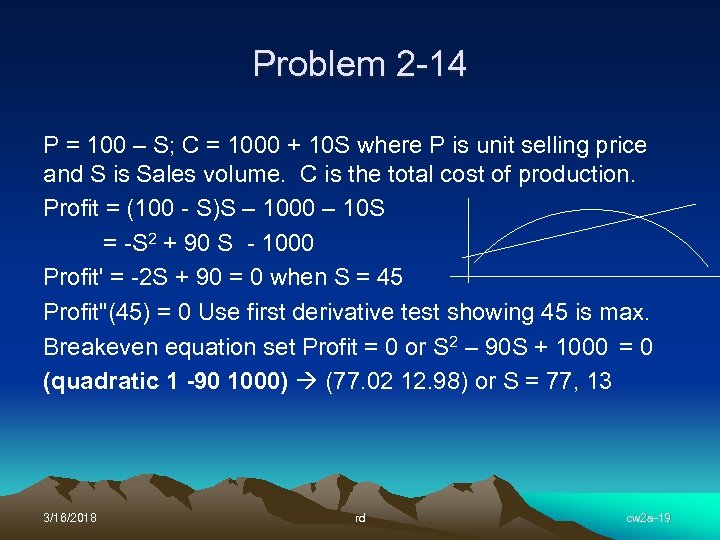Problem 2 -14 P = 100 – S; C = 1000 + 10 S where P is unit selling price and S is Sales volume. C is the total cost of production. Profit = (100 - S)S – 1000 – 10 S = -S 2 + 90 S - 1000 Profit' = -2 S + 90 = 0 when S = 45 Profit"(45) = 0 Use first derivative test showing 45 is max. Breakeven equation set Profit = 0 or S 2 – 90 S + 1000 = 0 (quadratic 1 -90 1000) (77. 02 12. 98) or S = 77, 13 3/16/2018 rd cw 2 a-19

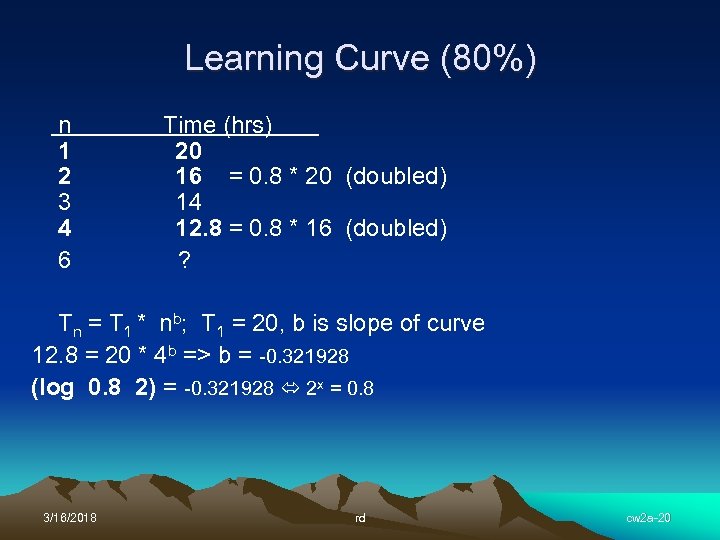Learning Curve (80%) n 1 2 3 4 6 Time (hrs) 20 16 = 0. 8 * 20 (doubled) 14 12. 8 = 0. 8 * 16 (doubled) ? Tn = T 1 * nb; T 1 = 20, b is slope of curve 12. 8 = 20 * 4 b => b = -0. 321928 (log 0. 8 2) = -0. 321928 2 x = 0. 8 3/16/2018 rd cw 2 a-20

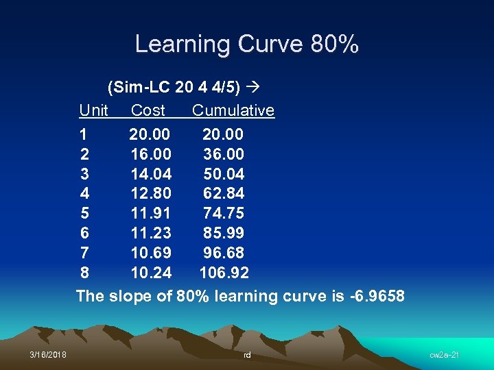Learning Curve 80% (Sim-LC 20 4 4/5) Unit Cost Cumulative 1 20. 00 2 16. 00 3 14. 04 50. 04 4 12. 80 62. 84 5 11. 91 74. 75 6 11. 23 85. 99 7 10. 69 96. 68 8 10. 24 106. 92 The slope of 80% learning curve is -6. 9658 3/16/2018 rd cw 2 a-21

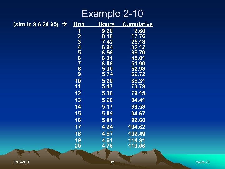Example 2 -10 (sim-lc 9. 6 20 85) 3/16/2018 Unit 1 2 3 4 5 6 7 8 9 10 11 12 13 14 15 16 17 18 19 20 Hours 9. 60 8. 16 7. 42 6. 94 6. 58 6. 31 6. 08 5. 90 5. 74 5. 60 5. 47 5. 36 5. 26 5. 17 5. 09 5. 01 4. 94 4. 87 4. 81 4. 76 rd Cumulative 9. 60 17. 76 25. 18 32. 12 38. 70 45. 01 51. 09 56. 98 62. 72 68. 31 73. 79 79. 15 84. 41 89. 58 94. 67 99. 68 104. 62 109. 49 114. 31 119. 06 cw 2 a-22

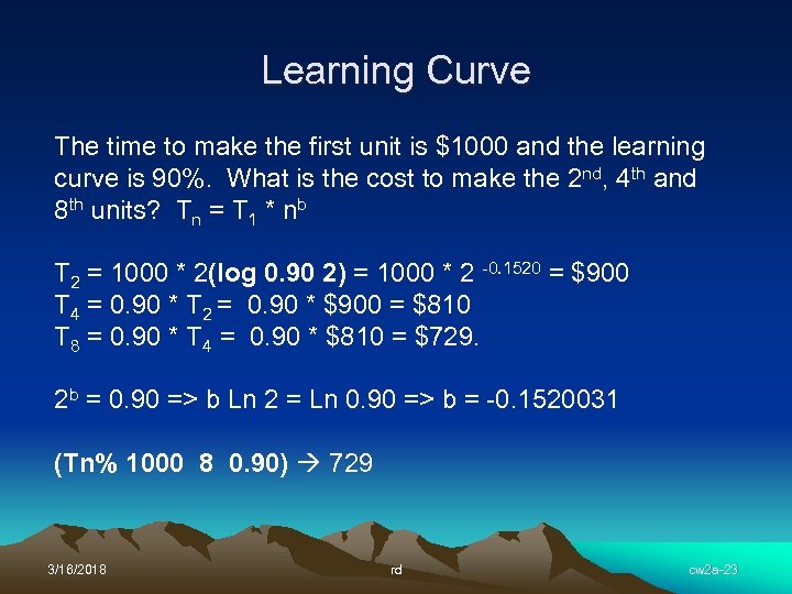Learning Curve The time to make the first unit is $1000 and the learning curve is 90%. What is the cost to make the 2 nd, 4 th and 8 th units? Tn = T 1 * nb T 2 = 1000 * 2(log 0. 90 2) = 1000 * 2 -0. 1520 = $900 T 4 = 0. 90 * T 2 = 0. 90 * $900 = $810 T 8 = 0. 90 * T 4 = 0. 90 * $810 = $729. 2 b = 0. 90 => b Ln 2 = Ln 0. 90 => b = -0. 1520031 (Tn% 1000 8 0. 90) 729 3/16/2018 rd cw 2 a-23

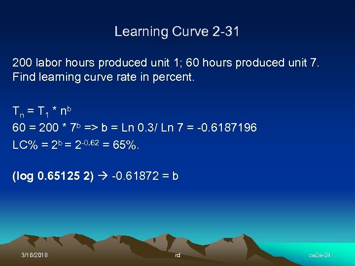Learning Curve 2 -31 200 labor hours produced unit 1; 60 hours produced unit 7. Find learning curve rate in percent. Tn = T 1 * n b 60 = 200 * 7 b => b = Ln 0. 3/ Ln 7 = -0. 6187196 LC% = 2 b = 2 -0. 62 = 65%. (log 0. 65125 2) -0. 61872 = b 3/16/2018 rd cw 2 a-24

Life Cycle Costs Concurrent Engineering Later the design changes, the more expensive the costs Early decisions lock in later costs. More accurate estimates Benefits usually overestimated Costs usually underestimated 3/16/2018 rd cw 2 a-25

Benefits vs. Costs Estimating Benefits – tend to be overestimated and accumulater in project. Costs – tend to be underestimated and mostly occur during beginning of project. 3/16/2018 rd cw 2 a-26

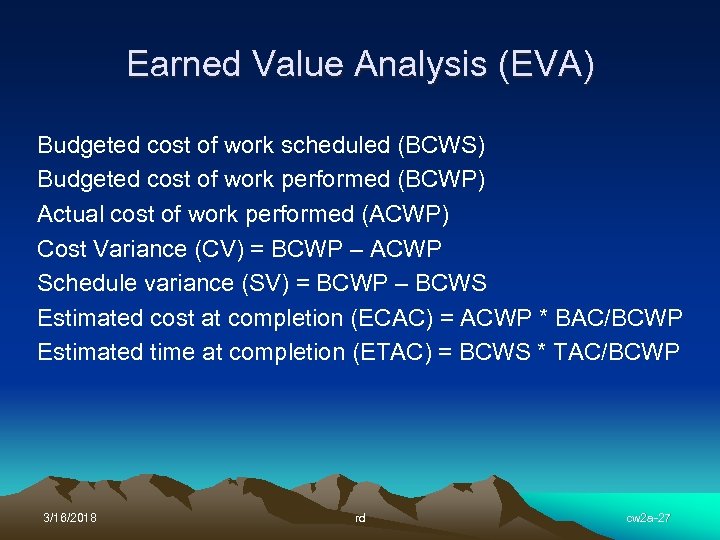Earned Value Analysis (EVA) Budgeted cost of work scheduled (BCWS) Budgeted cost of work performed (BCWP) Actual cost of work performed (ACWP) Cost Variance (CV) = BCWP – ACWP Schedule variance (SV) = BCWP – BCWS Estimated cost at completion (ECAC) = ACWP * BAC/BCWP Estimated time at completion (ETAC) = BCWS * TAC/BCWP 3/16/2018 rd cw 2 a-27

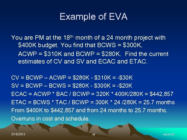Example of EVA You are PM at the 18 th month of a 24 month project with $400 K budget. You find that BCWS = $300 K, ACWP = $310 K and BCWP = $280 K. Find the current estimates of CV and SV and ECAC and ETAC. CV = BCWP – ACWP = $280 K - $310 K = -$30 K SV = BCWP – BCWS = $280 K - $300 K = -$20 K ECAC = ACWP * BAC / BCWP = 320 K * 400 K/280 K = $442, 857 ETAC = BCWS * TAC / BCWP = 300 K * 24 /280 K = 25. 7 months From $400 K to $442, 857 and from 24 months to 25. 7 months. Overruns in cost and schedule. 3/16/2018 rd cw 2 a-28

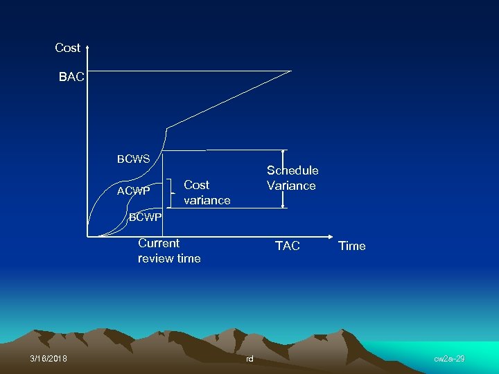Cost BAC BCWS ACWP Schedule Variance Cost variance BCWP Current review time 3/16/2018 TAC rd Time cw 2 a-29