Energy Planning Energy Economy Linkage Energy

Energy Planning

Energy Economy Linkage • Energy Consumption=F(Population, Activity Level, Energy Intensity. . . ) • E=(Energy/GDP)x(GDP/Capita)x. Pop • Gross Domestic Product proxy for Activity • Energy Intensity – dependent on Structre of Economy, energy efficiency • Energy critical input for development

Energy Planning • Dis-aggregation by sector • Dis-aggregation by end-use • Decide planning unit – village, town, state, nation, world • Decide planning horizon(base year , targetyear) • Need to have model

Load Forecasting / Energy Economy Models • Time Series Models • Input Output Models • Econometric Models • End-Use Models • Optimisation Framework • Accounting Framework

Uncertainties • Demand System • Supply Ø Ø Ø Equipment / System downtime Biomass Availability Supply variations • Weather

Load Profile • Consumers have usage patterns that vary with time • Load profile – aggregate pattern of all consumers • Peaks – Periods of maximum demand • Valleys – periods of manimum demand • Shoulders (Partial peak) - periods of intermediate demand

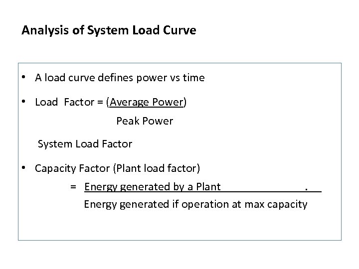Analysis of System Load Curve • A load curve defines power vs time • Load Factor = (Average Power) Peak Power System Load Factor • Capacity Factor (Plant load factor) = Energy generated by a Plant. Energy generated if operation at max capacity

Classification • Time intervals Ø Daily Load Curves (hourly/half hourly) Ø Seasonal (Winter/Summer/Monsoon) Ø Annual Load Curves • User classes Ø Residential Ø Industrial Ø Agricultural Ø Commercial • End Uses – Lighting, pumping, motors, heating, AC

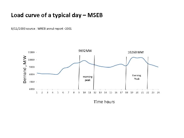Load curve of a typical day – MSEB 8/11/2000 source : WREB annul report -2001 Demand , M W 9892 MW Time hours

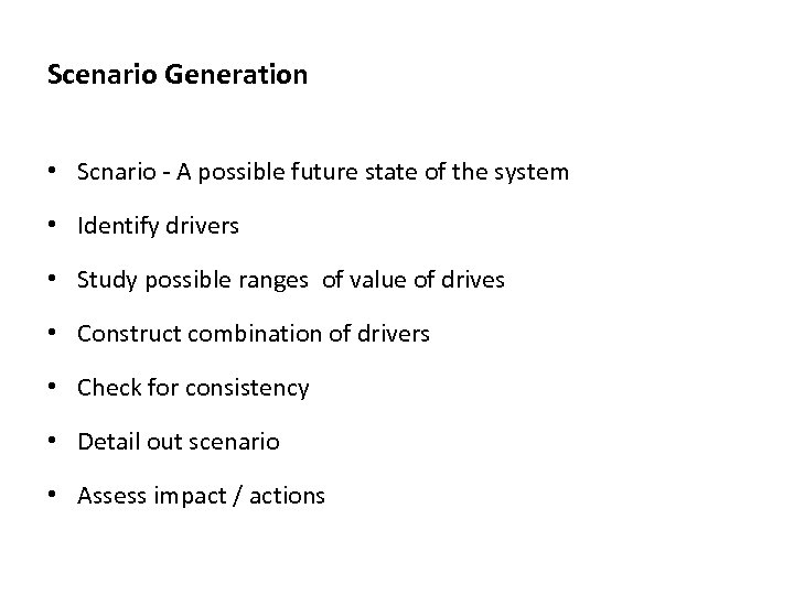Scenario Generation • Scnario - A possible future state of the system • Identify drivers • Study possible ranges of value of drives • Construct combination of drivers • Check for consistency • Detail out scenario • Assess impact / actions

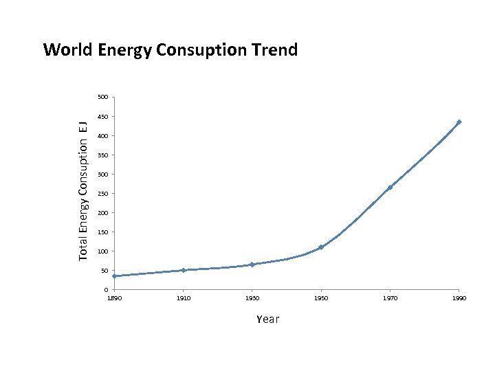World Energy Consuption Trend 500 Total Energy Consuption E J 450 400 350 300 250 200 150 100 50 0 1890 1910 1930 Year 1950 1970 1990

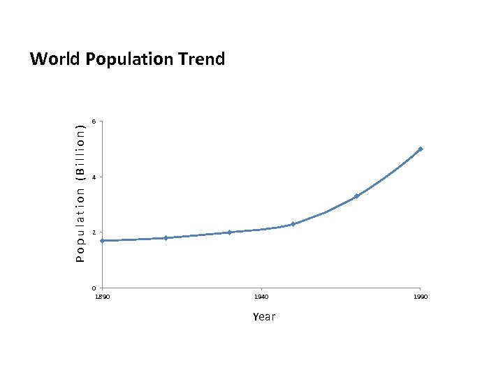Population (Billion) World Population Trend 6 4 2 0 1890 1940 Year 1990

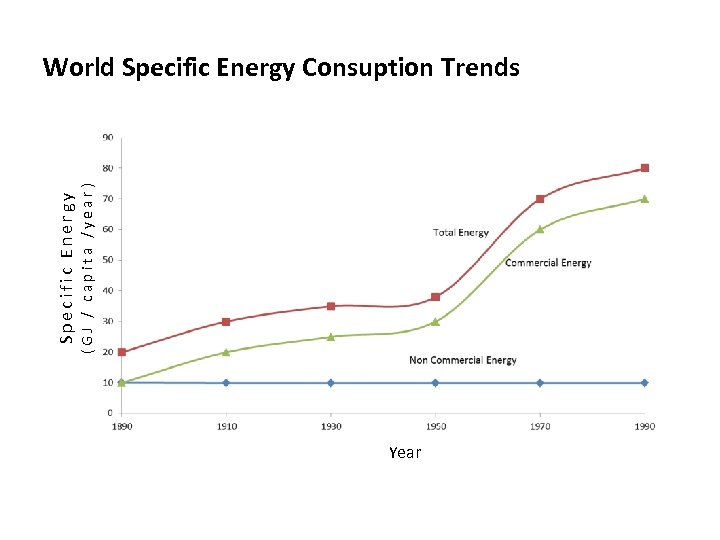Specific Energy (GJ / capita /year) World Specific Energy Consuption Trends Year

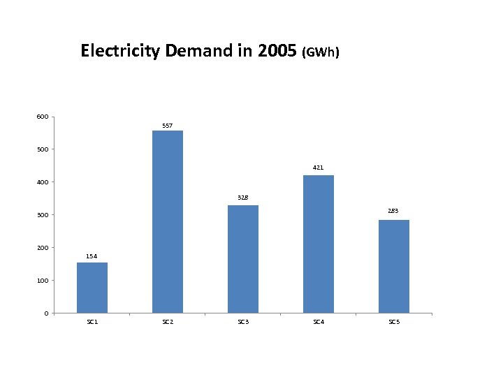
Electricity Demand Estimation • DST - UNDP project – Bankura district in West Bengal • Demand Scenarios • 1994 base year, Target year 2005 • Decion Support System for Energy planning

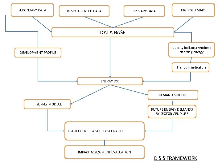SECONDARY DATA REMOTE SENSED DATA PRIMARY DATA DIGITISED MAPS DATA BASE Identity indicator/Variable affecting energy DEVELOPMENT PROFILE Trends in indicators ENERGY DSS DEMAND MODULE SUPPLY MODULE FUTURE ENERGY DEMANDS BY SECTOR / END USE FEASIBLE ENERGY SUPPLY SCENARIOS IMPACT ASSESSMENT EVALUATION D S S FRAMEWORK

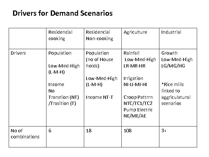Drivers for Demand Scenarios Residencial cooking Drivers Residencial Non-cooking Agriculture Population (no of House holds) Rainfall Growth Low-Med-High LR-MR-HR LG/MG/HG Low-Med-High (L-M-H) Irrigation NI-LI-MI-HI Income NT-T Croop Pattrrn NTC/TC 1/TC 2 Pump Electric NE/ME/AE 18 108 Low-Med-High (L-M-H) Income No Transtion (NT) /Trasition (T) No of combinations 6 Industrial *Rice mills linked to aggriculatural scenarios 3+

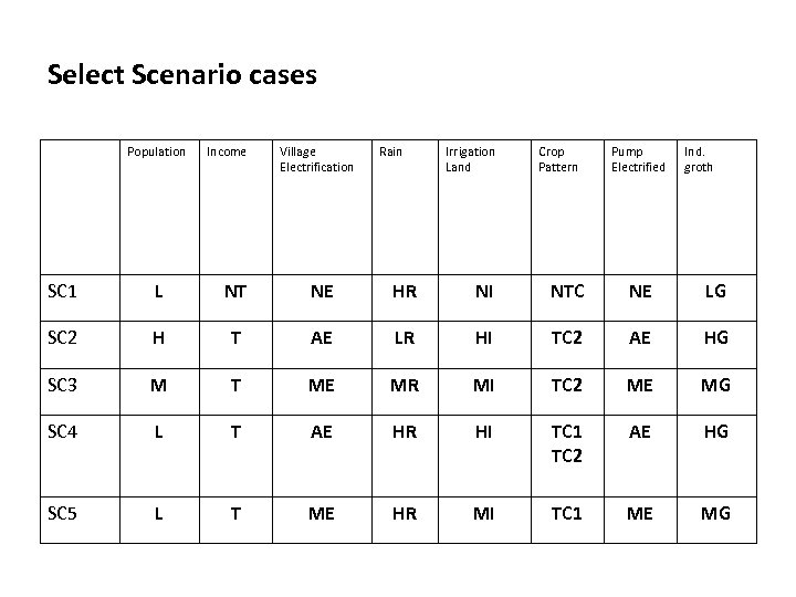Select Scenario cases Population Income Village Electrification Rain Irrigation Land Crop Pattern Pump Electrified Ind. groth SC 1 L NT NE HR NI NTC NE LG SC 2 H T AE LR HI TC 2 AE HG SC 3 M T ME MR MI TC 2 ME MG SC 4 L T AE HR HI TC 1 TC 2 AE HG SC 5 L T ME HR MI TC 1 ME MG

Electricity Demand in 2005 (GWh) 600 557 500 421 400 328 283 300 200 154 100 0 SC 1 SC 2 SC 3 SC 4 SC 5

Ground Truthing Remote Sensed images Crop residue factors GAS ANALYSIS Estimation of crop areas Digitized maps Map showing Landuse Classification Secondary Data Estimation of wood volume correlations Height, Density measurements Areal extent of forest nonforest Sub classification of Sal. And Mixed forests ACCOUNTING MODULE Standing wood estimate forest areas CROP RESIDUE MODULE Average fuelwood density nonforest(Survey/hterature) Fuel wood nonforest FUELWOOD MODULE Total fuelwood available Fuelwood available from forest areas ACCOUNTING MODULE Supply module for Biomass Estimation Total crop residues available % of Fuelwood

Demographics 1 Number of Households(HH) 2 % of HH in each income class Appliance ownership data by each income class Total no of Appliance in Area Technology Characteristics 1 Rating (k. W) 2 Effiency Usage Pattern 1 Daily variation 2 Seasonal variation Electricity consuption in Residential sector(including the load curve) for each seasona/Annual Number of Electric pump sets Agriculture load Usage and Seasonal variation Techanical specification Appliance ownership Number of commercial shops Total Appliances Tecnical Characteristics and usage Commercial load Total Electricity Demand. Daily load curve summer /Winter

Income class distribution in Rajamele in 1994 High Income; 13% Above Poverty; 31% Middle Income; 23% Below Poverty; 33%

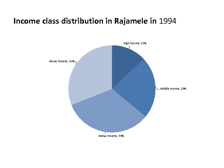
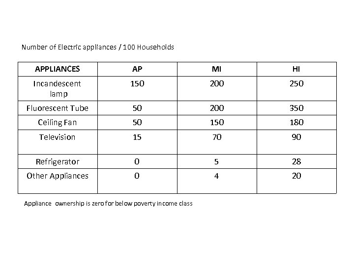Number of Electric appliances / 100 Households APPLIANCES AP MI HI Incandescent lamp 150 200 250 Fluorescent Tube 50 200 350 Ceiling Fan 50 180 Television 15 70 90 Refrigerator 0 5 28 Other Appliances 0 4 20 Appliance ownership is zero for below poverty income class

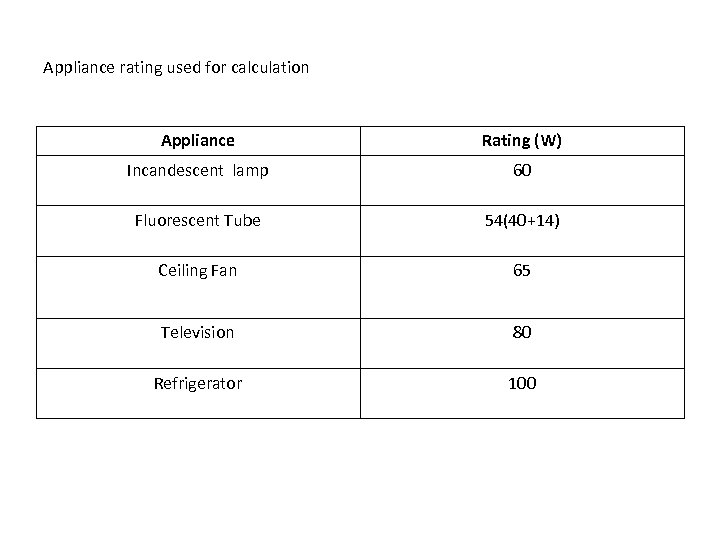Appliance rating used for calculation Appliance Rating (W) Incandescent lamp 60 Fluorescent Tube 54(40+14) Ceiling Fan 65 Television 80 Refrigerator 100

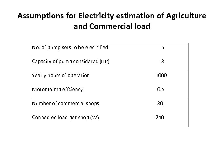Assumptions for Electricity estimation of Agriculture and Commercial load No. of pump sets to be electrified 5 Capacity of pump considered (HP) 3 Yearly hours of operation 1000 Motor Pump effciency 0. 5 Number of commercial shops 30 Connected load per shop (W) 240

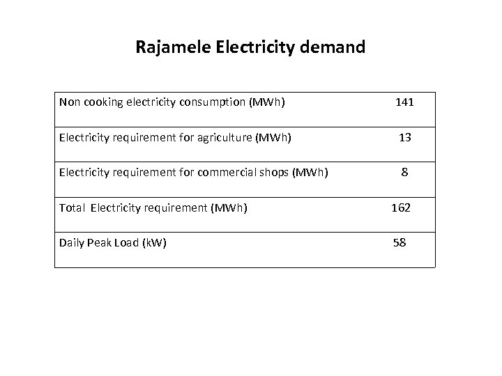Rajamele Electricity demand Non cooking electricity consumption (MWh) 141 Electricity requirement for agriculture (MWh) 13 Electricity requirement for commercial shops (MWh) 8 Total Electricity requirement (MWh) 162 Daily Peak Load (k. W) 58

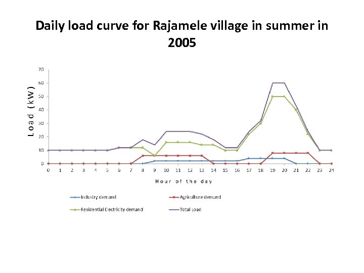Load (k. W) Daily load curve for Rajamele village in summer in 2005

Summing Up • Scenario generation – Useful tool for dealing with uncertainty • Models Useful for planing • Energy required critically depend on development profile • Matching of Supply –Demand • Dengers of over /Under estimates

End Note If a man begains with certainties , he will end in doubt, if he begins with doubts he will end in certainties. Anon

Emission Inventories

• An emission inventory is an accounting of the amount of pollutants discharged into the atmosphere. An emission inventory usually contains the total emissions for one or more specific GHGs or air pollutants, originating from all source categories in a certain geographical area and within a specified time span, usually a specific year. • An emission inventory is generally characterized by the following aspects: • • • Why: The types of activities that cause emissions, What: The chemical or physical identity of the pollutants included, Where: The geographic area covered, When: The time period over which emissions are estimated, How: The methodology to use.

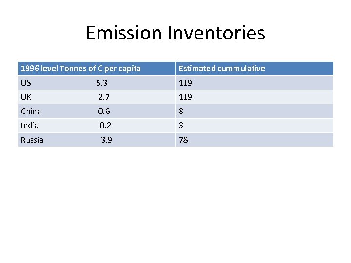Emission Inventories 1996 level Tonnes of C per capita Estimated cummulative US 5. 3 119 UK 2. 7 119 China 0. 6 8 India 0. 2 3 Russia 3. 9 78

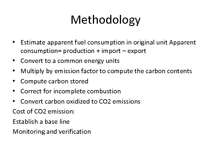Methodology • Estimate apparent fuel consumption in original unit Apparent consumption= production + import – export • Convert to a common energy units • Multiply by emission factor to compute the carbon contents • Compute carbon stored • Correct for incomplete combustion • Convert carbon oxidized to CO 2 emissions Cost of CO 2 emission: Establish a base line Monitoring and verification

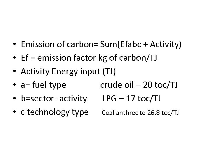• • • Emission of carbon= Sum(Efabc + Activity) Ef = emission factor kg of carbon/TJ Activity Energy input (TJ) a= fuel type crude oil – 20 toc/TJ b=sector- activity LPG – 17 toc/TJ c technology type Coal anthrecite 26. 8 toc/TJ