End of Chapter 10 ECON 151 PRINCIPLES

End of Chapter 10 ECON 151 – PRINCIPLES OF MACROECONOMICS Chapter 10 Chapter 11: Classical and Keynesian Macro Analyses Materials include content from Pearson Addison-Wesley which has been modified by the instructor and displayed with permission of the publisher. All rights reserved. 1 1

The Classical Model n The classical model was the first attempt to explain ¨ Determinants ¨ National of the price levels of real GDP ¨ Employment ¨ Consumption ¨ Saving ¨ Investment 11 -2

The Classical Model (cont'd) n Classical economists—Adam Smith, J. B. Say, David Ricardo, John Stuart Mill, Thomas Malthus, A. C. Pigou, and others— wrote from the 1770 s to the 1930 s. n They assumed wages and prices were flexible, and that competitive markets existed throughout the economy. 11 -3

The Classical Model (cont'd) n Say’s Law ¨A dictum of economist J. B. Say that supply creates its own demand ¨ Producing goods and services generates the means and the willingness to purchase other goods and services. ¨ Supply creates its own demand; hence it follows that desired expenditures will equal actual expenditures. 11 -4

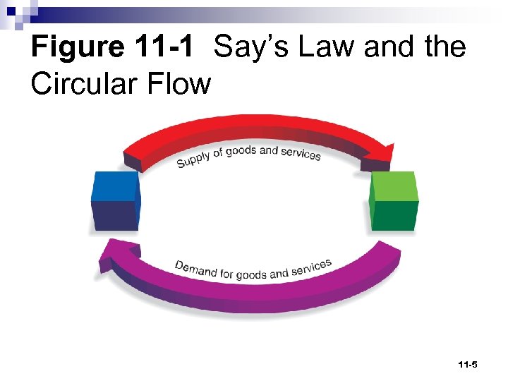Figure 11 -1 Say’s Law and the Circular Flow 11 -5

The Classical Model (cont'd) n Assumptions of the classical model ¨ Pure competition exists. ¨ Wages and prices are flexible. ¨ People are motivated by self-interest. ¨ People cannot be fooled by money illusion. 11 -6

The Classical Model (cont'd) n Money Illusion ¨ Reacting to changes in money prices rather than relative prices ¨ If a worker whose wages double when the price level also doubles thinks he or she is better off, that worker is suffering from money illusion. 11 -7

The Classical Model (cont'd) n Consequences of the assumptions ¨ If the role of government in the economy is minimal, ¨ If pure competition prevails, and all prices and wages are flexible, ¨ If people are self-interested, and do not experience money illusion, ¨ Then problems in the macroeconomy will be temporary and the market will correct itself. 11 -8

The Classical Model (cont'd) n Equilibrium in the credit market ¨ When income is saved, it is not reflected in product demand. ¨ It is a type of leakage from the circular flow of income and output, because saving withdraws funds from the income stream. 11 -9

The Classical Model (cont'd) n Equilibrium in the credit market ¨ Classical economists contended each dollar saved would be matched by business investment. ¨ Leakages would thus equal injections. ¨ At equilibrium, the price of credit—the interest rate—ensures that the amount of credit demanded equals the amount supplied. 11 -10

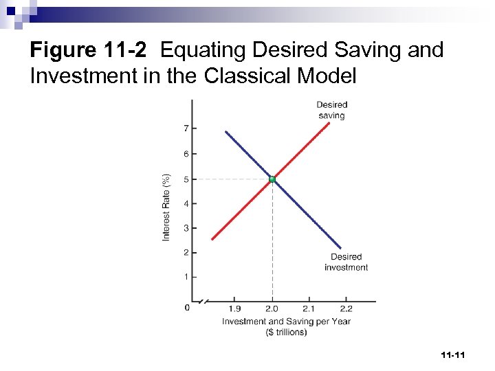Figure 11 -2 Equating Desired Saving and Investment in the Classical Model 11 -11

Equating Desired Saving and Investment in the Classical Model n Summary ¨ Changes in saving and investment create a surplus or shortage in the short run. ¨ In the long run, this is offset by changes in the interest rate. ¨ This interest rate adjustment returns the market to equilibrium where S = I. 11 -12

The Classical Model (cont'd) n Question ¨ Would unemployment be a problem in the classical model? n Answer ¨ No, classical economists assumed wages would always adjust to the full employment level. 11 -13

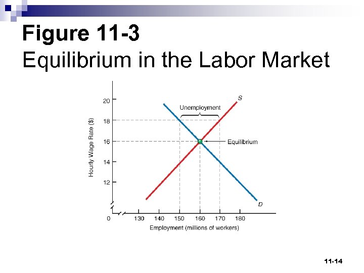Figure 11 -3 Equilibrium in the Labor Market 11 -14

Classical Theory, Vertical Aggregate Supply, and the Price Level n In the classical model, long-term unemployment is impossible. n Say’s law, coupled with flexible interest rates, prices, and wages would tend to keep workers fully employed. n The LRAS curve is vertical. n A change in aggregate demand will cause a change in the price level. 11 -15

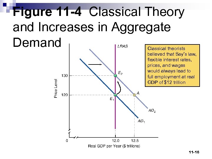Figure 11 -4 Classical Theory and Increases in Aggregate Demand Classical theorists believed that Say’s law, flexible interest rates, prices, and wages would always lead to full employment at real GDP of $12 trillion 11 -16

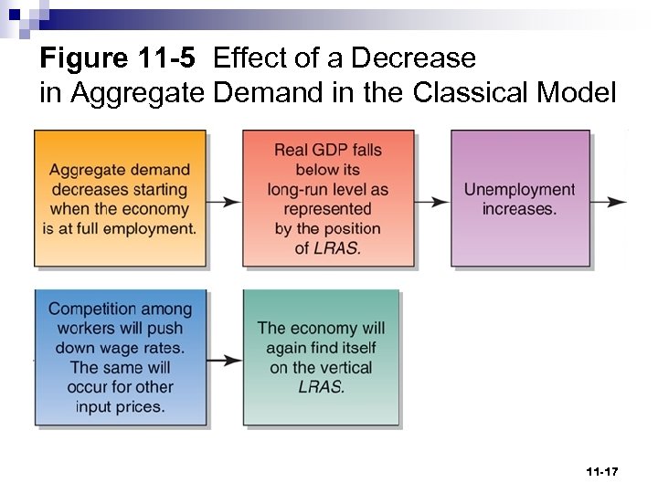Figure 11 -5 Effect of a Decrease in Aggregate Demand in the Classical Model 11 -17

Keynesian Economics and the Keynesian Short-Run Aggregate Supply Curve n The classical economists’ world was one of fully utilized resources. n In the 1930 s, Europe and the United States entered a period of economic decline that could not be explained by the classical model n John Maynard Keynes developed an explanation that has become known as the Keynesian model. 11 -18

Keynesian Economics and the Keynesian Short-Run Aggregate Supply Curve (cont'd) n Keynes and his followers argued ¨ Prices, including wages (the price of labor) are inflexible, or “sticky”, downward ¨ An increase in aggregate demand, AD, will not raise the price level ¨A decrease in AD will not cause firms to lower the price level 11 -19

Keynesian Economics and the Keynesian Short-Run Aggregate Supply Curve (cont'd) n Keynesian Short-Run Aggregate Supply Curve ¨ The horizontal portion of the aggregate supply curve in which there is excessive unemployment and unused capacity in the economy 11 -20

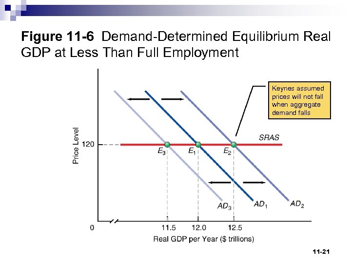Figure 11 -6 Demand-Determined Equilibrium Real GDP at Less Than Full Employment Keynes assumed prices will not fall when aggregate demand falls 11 -21

Keynesian Economics and the Keynesian Short-Run Aggregate Supply Curve (cont'd) n Real GDP and the price level, 1934– 1940 ¨ Keynes argued that in a depressed economy, increased aggregate spending can increase output without raising prices. ¨ Data showing the U. S. recovery from the Great Depression seem to bear this out. ¨ In such circumstances, real GDP is demand driven. 11 -22

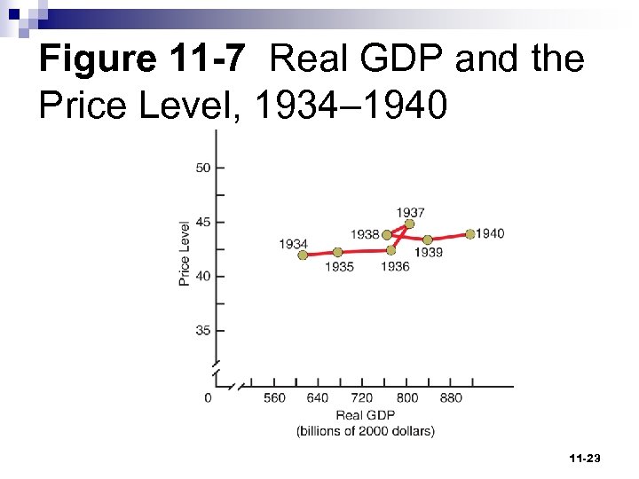Figure 11 -7 Real GDP and the Price Level, 1934– 1940 11 -23

Keynesian Economics and the Keynesian Short. Run Aggregate Supply Curve (cont'd) n The Keynesian model ¨ Equilibrium GDP is demand-determined. (Recall that under classical theory according to Say’s Law, the equilibrium is supply driven – supply creates its own demand. ) ¨ The Keynesian short-run aggregate supply schedule shows sources of price rigidities. n Union and long-term contracts explain inflexibility of nominal wage rates. 11 -24

Example: Bringing Keynesian Short-Run Aggregate Supply Back to Life n New Keynesians contend the SRAS curve is essentially flat. n Based on research, they contend SRAS is horizontal because firms adjust their prices about once a year. n The underlying assumption of the simplified Keynesian model is that the relevant range of the short-run aggregate supply schedule (SRAS) is horizontal. 11 -25

Output Determination Using Aggregate Demand Aggregate Supply: Fixed versus Changing Price Levels in the Short Run (cont'd) n The price level has drifted upward in recent decades. n Prices are not totally sticky. n Modern Keynesian analysis recognizes some—but not complete—price adjustment takes place in the short run. 11 -26

Output Determination Using Aggregate Demand Aggregate Supply: Fixed versus Changing Price Levels in the Short Run (cont'd) n Short-Run Aggregate Supply Curve ¨ Relationship between total planned economywide production and the price level in the short run, all other things held constant ¨ If prices adjust incompletely in the short run, the curve is positively sloped. 11 -27

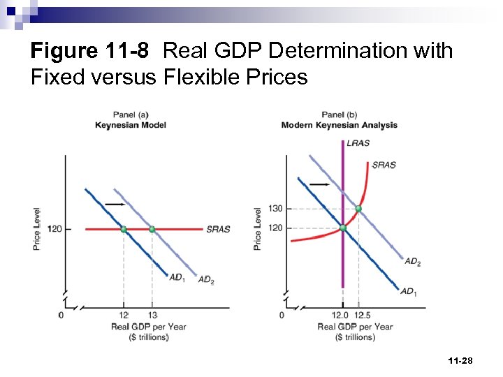Figure 11 -8 Real GDP Determination with Fixed versus Flexible Prices 11 -28

Output Determination Using Aggregate Demand Aggregate Supply: Fixed versus Changing Price Levels in the Short Run (cont'd) n In modern Keynesian short run, when the price level rises partially, real GDP can be expanded beyond the level consistent with its long-run growth path. 11 -29

Output Determination Using Aggregate Demand Aggregate Supply: Fixed versus Changing Price Levels in the Short Run (cont'd) n All these adjustments cause real GDP to rise as the price level increases ¨ Firms use workers more intensively, (getting workers to work harder) ¨ Existing capital equipment used more intensively, (use machines longer) ¨ If wage rates held constant, a higher price level leads to increased profits, which leads to lower unemployment as firms hire more 11 -30

Shifts in the Aggregate Supply Curve n Just as non-price-level factors can cause a shift in the aggregate demand curve, there are non-price-level factors that can cause a shift in the aggregate supply curve. n Shifts in both the short- and long-run aggregate supply n Shifts in SRAS only 11 -31

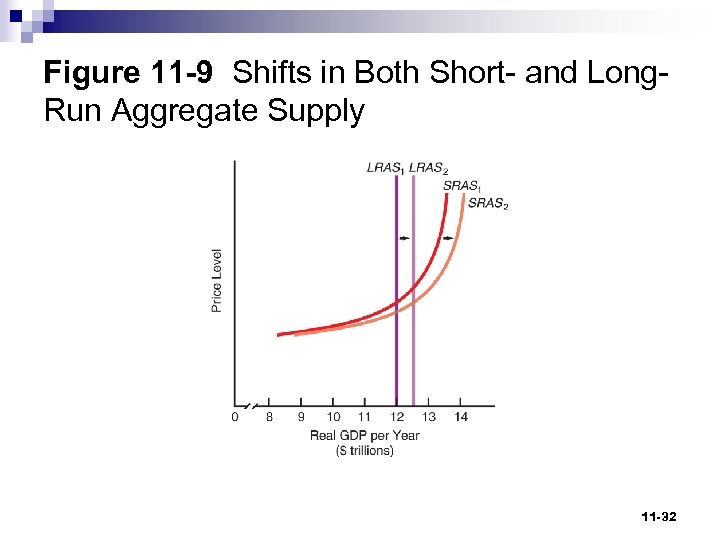Figure 11 -9 Shifts in Both Short- and Long. Run Aggregate Supply 11 -32

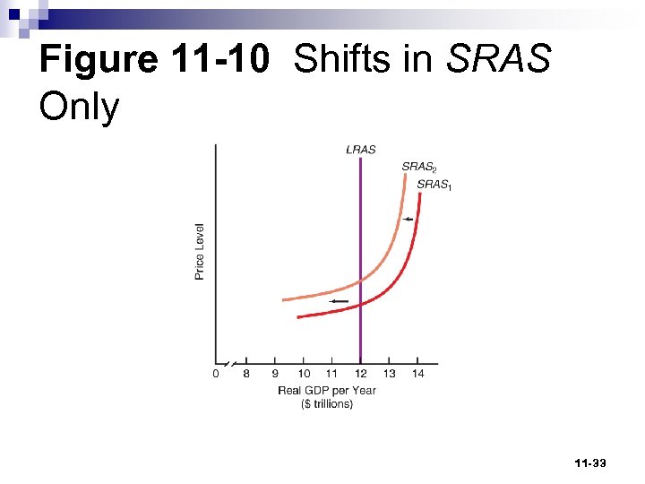Figure 11 -10 Shifts in SRAS Only 11 -33

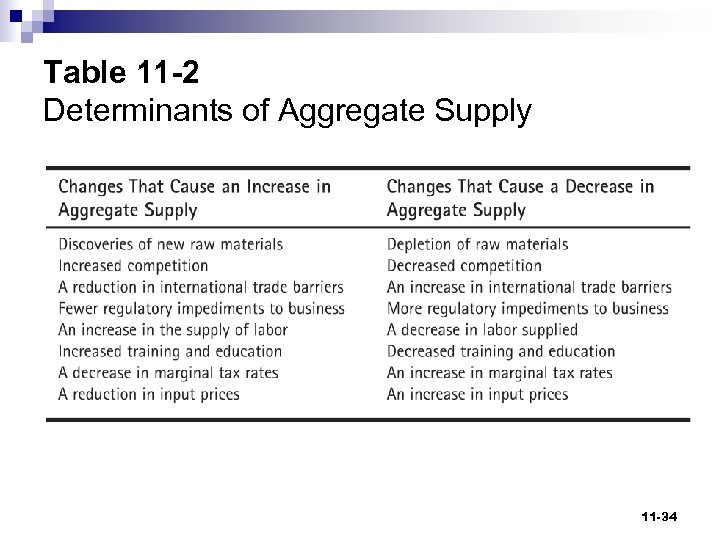Table 11 -2 Determinants of Aggregate Supply 11 -34

Consequences of Changes in Aggregate Demand Shock ¨ Any event that causes the aggregate demand curve to shift inward or outward n Aggregate Supply Shock ¨ Any event that causes the aggregate supply curve to shift inward or outward 11 -35

Consequences of Changes in Aggregate Demand n Recessionary Gap ¨ The gap that exists whenever equilibrium real GDP per year is less than full-employment real GDP as shown by the position of the LRAS curve n Inflationary Gap ¨ The gap that exists whenever equilibrium real GDP per year is greater than full-employment real GDP as shown by the position of the LRAS curve 11 -36

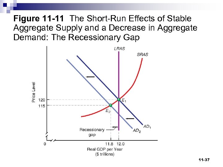Figure 11 -11 The Short-Run Effects of Stable Aggregate Supply and a Decrease in Aggregate Demand: The Recessionary Gap 11 -37

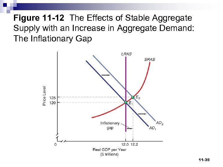Figure 11 -12 The Effects of Stable Aggregate Supply with an Increase in Aggregate Demand: The Inflationary Gap 11 -38

Explaining Short-Run Variations in Inflation n In a growing economy, the explanation for persistent inflation is that aggregate demand rises over time at a faster pace than the full-employment level of real GDP. n Short-run variations in inflation, however, can arise as a result of both demand supply factors. 11 -39

Explaining Short-Run Variations in Inflation (cont'd) n Demand-Pull Inflation ¨ Inflation caused by increases in aggregate demand not matched by increases in aggregate supply n Cost-Push Inflation ¨ Inflation caused by decreases in short-run aggregate supply 11 -40

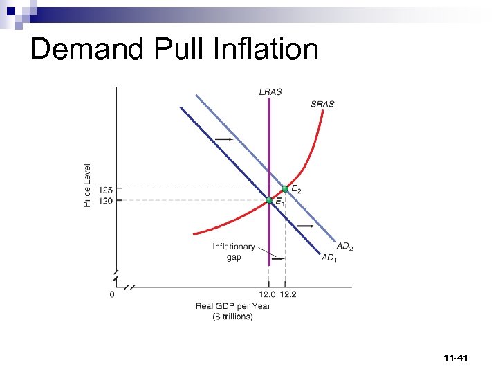Demand Pull Inflation 11 -41

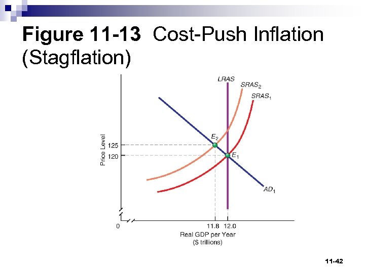Figure 11 -13 Cost-Push Inflation (Stagflation) 11 -42

Aggregate Demand Supply in an Open Economy n The open economy is one of the reasons why aggregate demand slopes downward. ¨ When the domestic price level rises, U. S. residents want to buy cheaper-priced foreign goods. ¨ The opposite occurs when the U. S. domestic price level falls. 11 -43

Aggregate Demand Supply in an Open Economy (cont'd) n Currently, the foreign sector of the U. S. economy constitutes over 14% of all economic activities. 11 -44

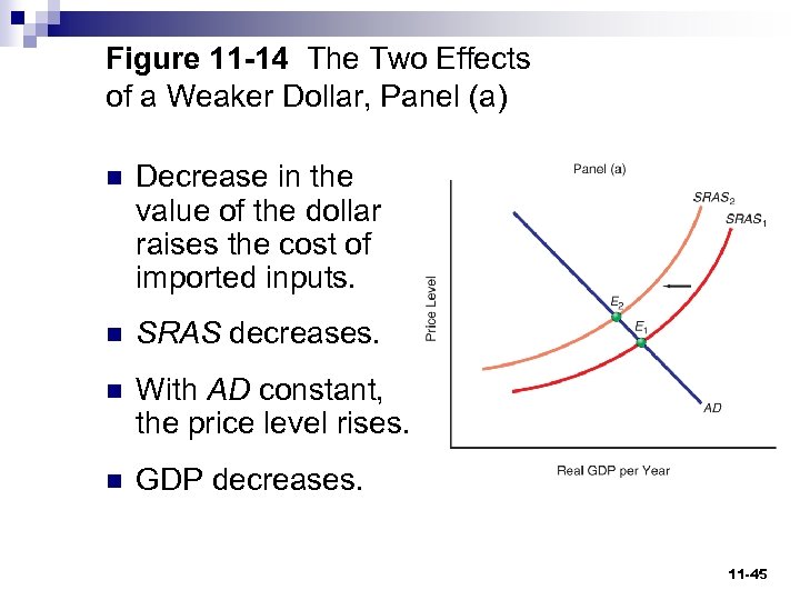Figure 11 -14 The Two Effects of a Weaker Dollar, Panel (a) n Decrease in the value of the dollar raises the cost of imported inputs. n SRAS decreases. n With AD constant, the price level rises. n GDP decreases. 11 -45

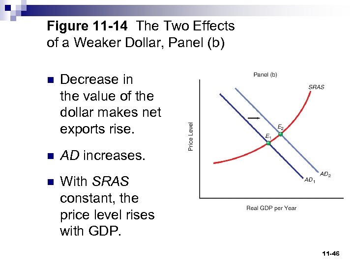Figure 11 -14 The Two Effects of a Weaker Dollar, Panel (b) n Decrease in the value of the dollar makes net exports rise. n AD increases. n With SRAS constant, the price level rises with GDP. 11 -46

End of Chapter 10 ECON 151 – PRINCIPLES OF MACROECONOMICS Chapter 10 Chapter 11: Classical and Keynesian Macro Analyses Materials include content from Pearson Addison-Wesley which has been modified by the instructor and displayed with permission of the publisher. All rights reserved. 47 47