ENCI 303 Lecture PS-18 Optimization 1 Overview

ENCI 303 Lecture PS-18 Optimization 1

Overview of lecture § Introduction and examples. § The optimization framework. ENCI 303 Lecture PS-18 Optimization 1 18 -2 Glory to You! § The Excel Solver.

Introduction and examples (1) § Goal of optimization is to find values of the design variables that maximize or minimize an objective function, possibly with constraints on the design variables. § Example: A textile factory makes fabrics with different colours. It has a high quality dyeing machine but with limited capacity, and so has to subcontract some of its dyeing operations. The different coloured fabrics cost different amounts to dye, whether in-house or subcontracted, and they are sold at different prices. ENCI 303 Lecture PS-18 Optimization 1 18 -3 Glory to You! Problem: How much of each coloured fabric should be subcontracted so as to maximize profit?

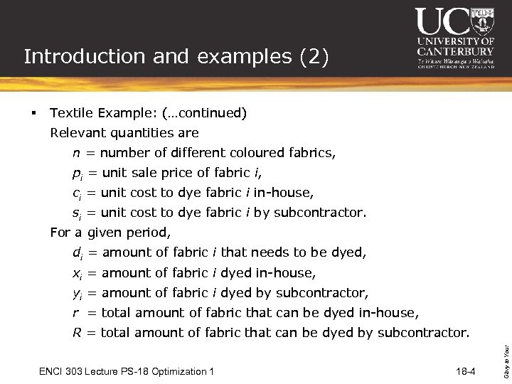Introduction and examples (2) Textile Example: (…continued) Relevant quantities are n = number of different coloured fabrics, pi = unit sale price of fabric i, ci = unit cost to dye fabric i in-house, si = unit cost to dye fabric i by subcontractor. For a given period, di = amount of fabric i that needs to be dyed, xi = amount of fabric i dyed in-house, yi = amount of fabric i dyed by subcontractor, r = total amount of fabric that can be dyed in-house, R = total amount of fabric that can be dyed by subcontractor. ENCI 303 Lecture PS-18 Optimization 1 18 -4 Glory to You! §

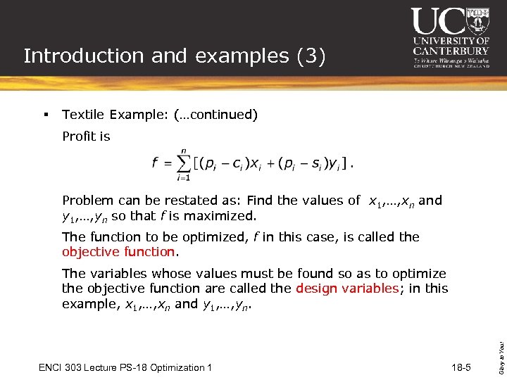Introduction and examples (3) § Textile Example: (…continued) Profit is Problem can be restated as: Find the values of x 1, …, xn and y 1, …, yn so that f is maximized. The function to be optimized, f in this case, is called the objective function. ENCI 303 Lecture PS-18 Optimization 1 18 -5 Glory to You! The variables whose values must be found so as to optimize the objective function are called the design variables; in this example, x 1, …, xn and y 1, …, yn.

Introduction and examples (4) § Textile Example: (…continued) There may be constraints on the design variables, restricting the possible values that they can have. In this example, the constraints on x 1, …, xn and y 1, …, yn are xi + yi = di , i = 1, …, n x 1 + + xn r y 1 + + yn R ENCI 303 Lecture PS-18 Optimization 1 18 -6 Glory to You! xi , yi 0 , i = 1, …, n.

Introduction and examples (5) § Textile Example: (…continued) Complete statement of the optimization problem: Find x 1, …, xn and y 1, …, yn to maximize subject to xi + yi = di , i = 1, …, n x 1 + + xn r y 1 + + yn R ENCI 303 Lecture PS-18 Optimization 1 18 -7 Glory to You! xi , yi 0 , i = 1, …, n.

Introduction and examples (6) § Example: Transportation problem. m supply points where quantities, s 1, …, sm, are produced or stocked. n destinations where quantities, d 1, …, dn, are in demand. Cost cij is incurred on an item shipped from supply point i to destination j. Amount xij shipped from supply point i to destination j. ENCI 303 Lecture PS-18 Optimization 1 18 -8 Glory to You! Problem: Find the amounts that must be shipped from each supply point to each destination so as to minimize total cost.

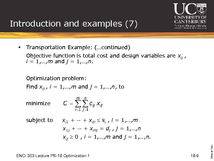Introduction and examples (7) § Transportation Example: (…continued) Objective function is total cost and design variables are xij , i = 1, …, m and j = 1, …, n. Optimization problem: Find xij , i = 1, …, m and j = 1, …, n, to minimize subject to xi 1 + + xin si , i = 1, …, m x 1 j + + xmj = dj , j = 1, …, n ENCI 303 Lecture PS-18 Optimization 1 18 -9 Glory to You! xij 0 , i = 1, …, m and j = 1, …, n.

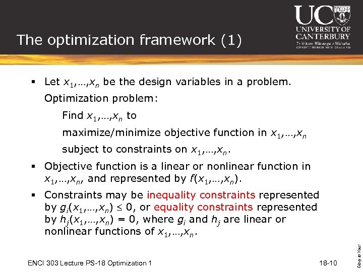The optimization framework (1) § Let x 1, …, xn be the design variables in a problem. Optimization problem: Find x 1, …, xn to maximize/minimize objective function in x 1, …, xn subject to constraints on x 1, …, xn. § Objective function is a linear or nonlinear function in x 1, …, xn, and represented by f(x 1, …, xn). ENCI 303 Lecture PS-18 Optimization 1 18 -10 Glory to You! § Constraints may be inequality constraints represented by gi(x 1, …, xn) 0, or equality constraints represented by hj(x 1, …, xn) = 0, where gi and hj are linear or nonlinear functions of x 1, …, xn.

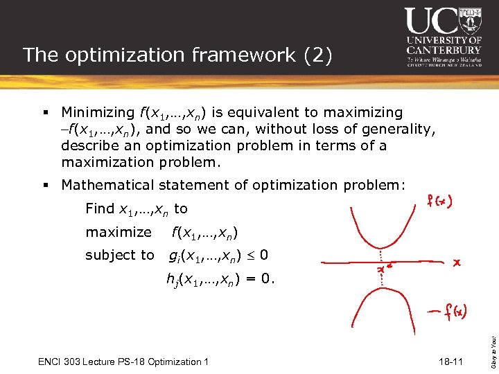The optimization framework (2) § Minimizing f(x 1, …, xn) is equivalent to maximizing f(x 1, …, xn), and so we can, without loss of generality, describe an optimization problem in terms of a maximization problem. § Mathematical statement of optimization problem: Find x 1, …, xn to maximize f(x 1, …, xn) subject to gi(x 1, …, xn) 0 ENCI 303 Lecture PS-18 Optimization 1 18 -11 Glory to You! hj(x 1, …, xn) = 0.

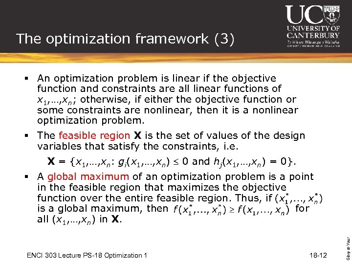The optimization framework (3) § An optimization problem is linear if the objective function and constraints are all linear functions of x 1, …, xn; otherwise, if either the objective function or some constraints are nonlinear, then it is a nonlinear optimization problem. § The feasible region X is the set of values of the design variables that satisfy the constraints, i. e. X = {x 1, …, xn: gi(x 1, …, xn) 0 and hj(x 1, …, xn) = 0}. ENCI 303 Lecture PS-18 Optimization 1 18 -12 Glory to You! § A global maximum of an optimization problem is a point in the feasible region that maximizes the objective function over the entire feasible region. Thus, if is a global maximum, then for all (x 1, …, xn) in X.

The optimization framework (4) § Ideally, we want to find a unique global maximum for our optimization problem. In practice, two difficulties may be encountered: § There may be more than one global maximum. Choose any one of them or use some other considerations to choose one of them. ENCI 303 Lecture PS-18 Optimization 1 18 -13 Glory to You! § A local maximum may be found instead of a global one. A local maximum is a point in the feasible region that maximizes the objective function in a neighbourhood around that point but not in the entire feasible region.

The Excel Solver (1) § The Excel Solver is a tool for solving linear and nonlinear optimization problems. § For linear optimization problems: Simplex method, with branch and bound algorithm for integer design variables. § For nonlinear optimization problems: Generalized reduced gradient method. § Launching the Excel Solver: Start the Excel program. ENCI 303 Lecture PS-18 Optimization 1 18 -14 Glory to You! Tools > Solver…

The Excel Solver (2) § Using the Excel Solver: Set Target Cell: Address of cell containing the formula for the objective function. Equal To: Choose Max for maximization problem or Min for minimization problem. By Changing Cells: Addresses of cells for the design variables. Subject to the Constraints: ENCI 303 Lecture PS-18 Optimization 1 18 -15 Glory to You! Choose Add to add a new constraint, Edit to change an existing constraint or Delete to delete an existing constraint.

The Excel Solver (3) § Using the Excel Solver: (…continued) Add: (adding a new constraint) Cell Reference: Address of design variable. Choose type of constraint: or = or int (integer) or bin (binary). Constraint: Value of constraint (if applicable). Options: Assume Non-Negative (if all design variables are nonnegative) > OK. ENCI 303 Lecture PS-18 Optimization 1 18 -16 Glory to You! OK or Add (to add another constraint)

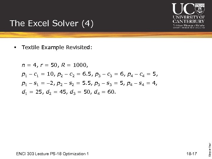The Excel Solver (4) § Textile Example Revisited: n = 4, r = 50, R = 1000, p 1 c 1 = 10, p 2 c 2 = 6. 5, p 3 c 3 = 6, p 4 c 4 = 5, p 1 s 1 = 2, p 2 s 2 = 5. 5, p 3 s 3 = 5, p 4 s 4 = 4, ENCI 303 Lecture PS-18 Optimization 1 18 -17 Glory to You! d 1 = 25, d 2 = 45, d 3 = 50, d 4 = 60.

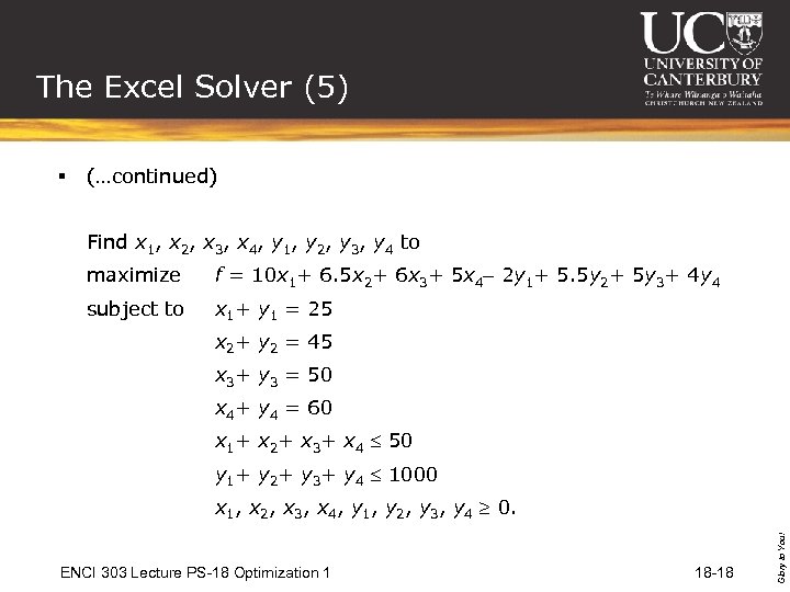The Excel Solver (5) § (…continued) Find x 1, x 2, x 3, x 4, y 1, y 2, y 3, y 4 to maximize f = 10 x 1+ 6. 5 x 2+ 6 x 3+ 5 x 4 2 y 1+ 5. 5 y 2+ 5 y 3+ 4 y 4 subject to x 1+ y 1 = 25 x 2+ y 2 = 45 x 3+ y 3 = 50 x 4+ y 4 = 60 x 1+ x 2+ x 3+ x 4 50 y 1+ y 2+ y 3+ y 4 1000 ENCI 303 Lecture PS-18 Optimization 1 18 -18 Glory to You! x 1, x 2, x 3, x 4, y 1, y 2, y 3, y 4 0.

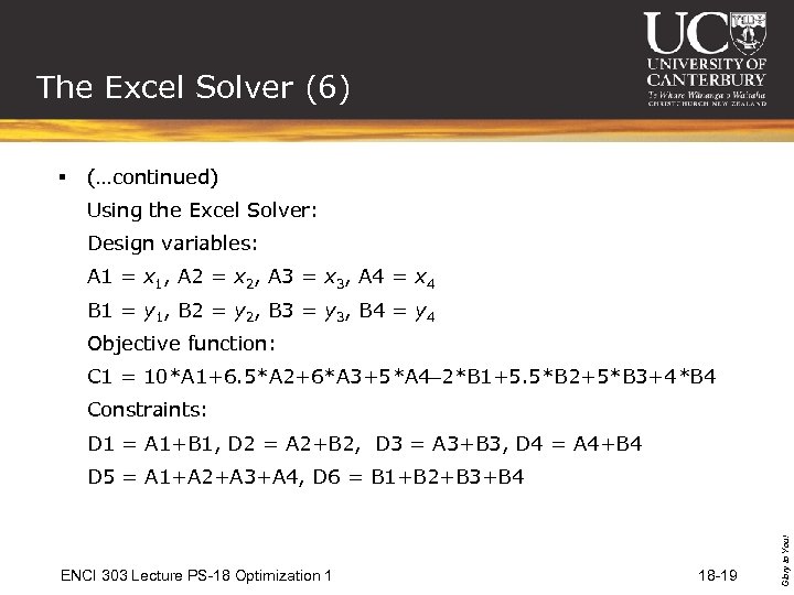The Excel Solver (6) § (…continued) Using the Excel Solver: Design variables: A 1 = x 1, A 2 = x 2, A 3 = x 3, A 4 = x 4 B 1 = y 1, B 2 = y 2, B 3 = y 3, B 4 = y 4 Objective function: C 1 = 10*A 1+6. 5*A 2+6*A 3+5*A 4 2*B 1+5. 5*B 2+5*B 3+4*B 4 Constraints: D 1 = A 1+B 1, D 2 = A 2+B 2, D 3 = A 3+B 3, D 4 = A 4+B 4 ENCI 303 Lecture PS-18 Optimization 1 18 -19 Glory to You! D 5 = A 1+A 2+A 3+A 4, D 6 = B 1+B 2+B 3+B 4

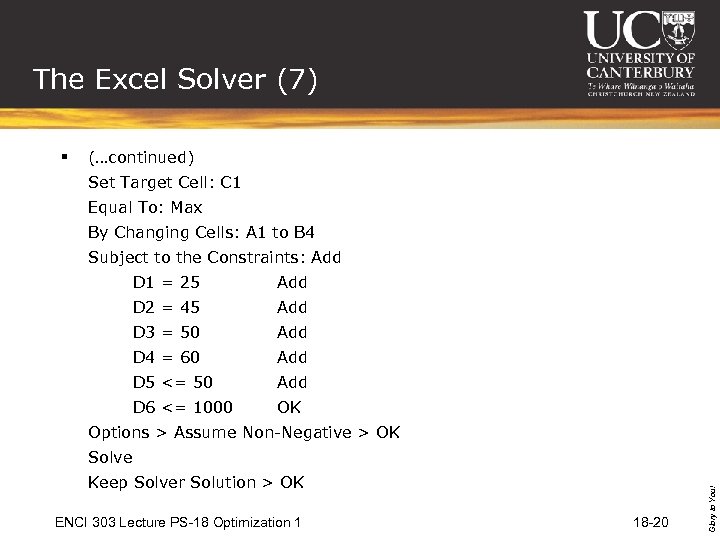The Excel Solver (7) § (…continued) Set Target Cell: C 1 Equal To: Max By Changing Cells: A 1 to B 4 Subject to the Constraints: Add D 1 = 25 Add D 2 = 45 Add D 3 = 50 Add D 4 = 60 Add D 5 <= 50 Add D 6 <= 1000 OK Options > Assume Non-Negative > OK Keep Solver Solution > OK ENCI 303 Lecture PS-18 Optimization 1 18 -20 Glory to You! Solve

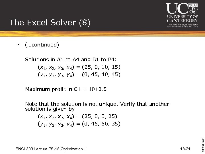The Excel Solver (8) § (…continued) Solutions in A 1 to A 4 and B 1 to B 4: (x 1, x 2, x 3, x 4) = (25, 0, 15) (y 1, y 2, y 3, y 4) = (0, 45, 40, 45) Maximum profit in C 1 = 1012. 5 ENCI 303 Lecture PS-18 Optimization 1 18 -21 Glory to You! Note that the solution is not unique. Verify that another solution is given by (x 1, x 2, x 3, x 4) = (25, 0, 0, 25) (y 1, y 2, y 3, y 4) = (0, 45, 50, 35)