Empirical temperature downscaling Improving thermal information detail David

Empirical temperature downscaling: Improving thermal information detail David E. Atkinson International Arctic Research Center Department of Atmospheric Sciences University of Alaska Fairbanks

The Problem High latitude regions are: > large > topographically complex and diverse > poorly serviced by weather instrumentation Problematic for users who require spatially detailed temperature > biological energetics > plants > hibernation energetics > cryological concerns > glacier melt > permafrost modeling > hydrology > limnology > paleoclimatic work > establish current temperature regime

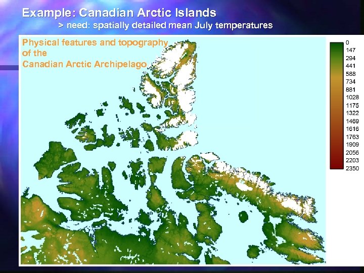Example: Canadian Arctic Islands > need: spatially detailed mean July temperatures Physical features and topography of the Canadian Arctic Archipelago meters ASL

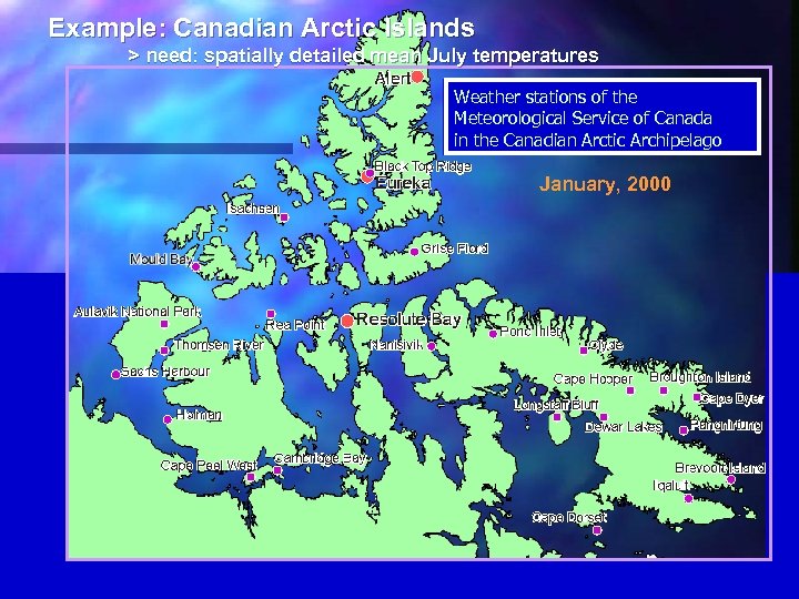Example: Canadian Arctic Islands > need: spatially detailed mean July temperatures Weather stations of the Meteorological Service of Canada in the Canadian Arctic Archipelago January, 2000

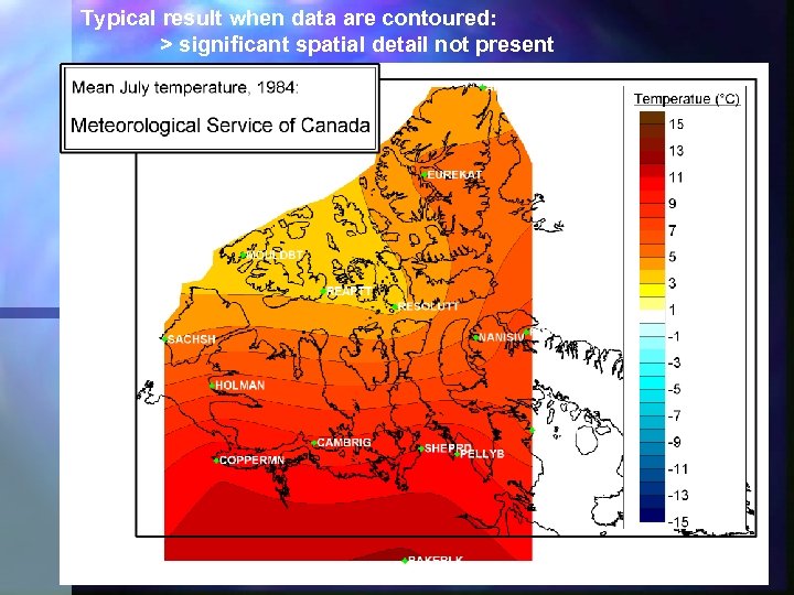Typical result when data are contoured: > significant spatial detail not present

Need Improve spatial detail for surface air temperature Options include: > targeted monitoring networks > dynamical weather models > empirical models Focus here on an empirical modeling solution to calculate surface air temperature at high spatial resolution

Definition An “Empirical” or distributed model: > uses information about location to improve interpolation Does not “generate” original data - works with existing estimates > weather stations or model input

Topoclimate Model v 2. 0 (2007) Atkinson and Francois Gourand (MA student, Meteo. France) Input data sources Digital Elevation Model - GTOPO 30 n NOAA National Weather Service GFS 0. 5 model inputs: n n @ Surface n n n @ Standard reporting levels n n n SLP Lup, Kdn T, u, v, cloud water Total cloudiness Surface weather observations n (for correction of final estimate - sfc obs are not used to develop the temperature estimate)

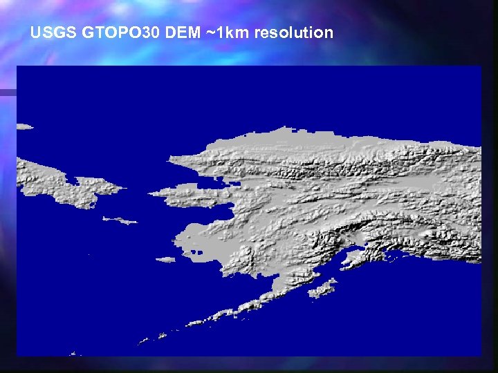USGS GTOPO 30 DEM ~1 km resolution

Topoclimate Model v 2. 0 (2007) Atkinson and Francois Gourand (MA student, Meteo. France) Input data sources Digital Elevation Model - GTOPO 30 n NOAA National Weather Service GFS 0. 5 model inputs: n n @ Surface n n n @ Standard reporting levels n n n SLP Lup, Kdn T, u, v, cloud water Total cloudiness Surface weather observations n (for correction of final estimate - sfc obs are not used to develop the temperature estimate)

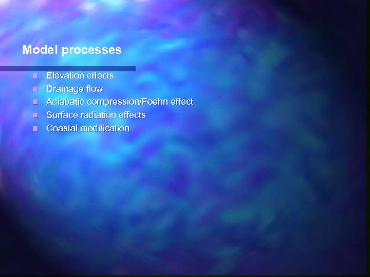Model processes n n n Elevation effects Drainage flow Adiabatic compression/Foehn effect Surface radiation effects Coastal modification

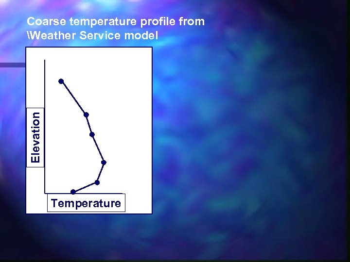Elevation Coarse temperature profile from Weather Service model Temperature

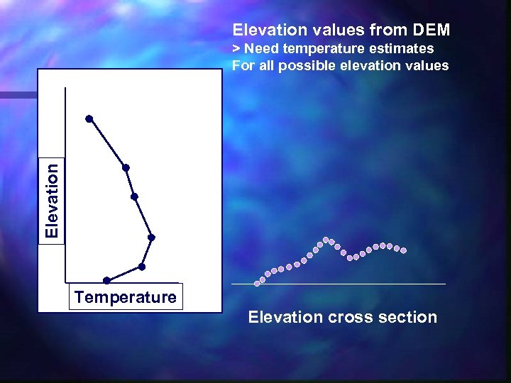Elevation values from DEM Elevation > Need temperature estimates For all possible elevation values Temperature Elevation cross section

Represent using a function > solve for T at all possible values of elevation > one T estimate for every pixel on the DEM Elevation T = B 0 + B 1*E + B 2*E 2 … etc Temperature

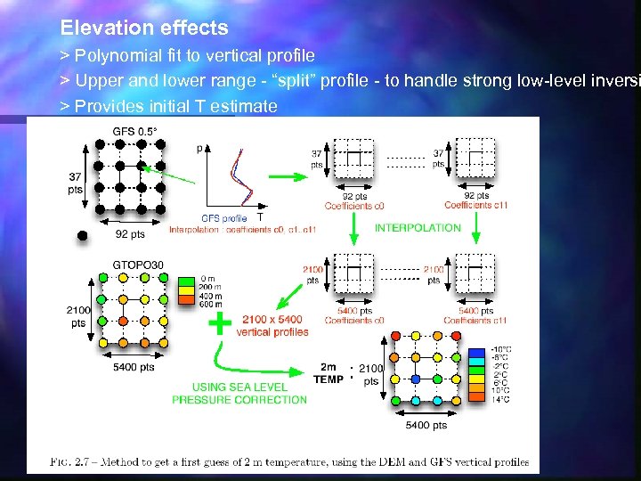Elevation effects > Polynomial fit to vertical profile > Upper and lower range - “split” profile - to handle strong low-level inversi > Provides initial T estimate

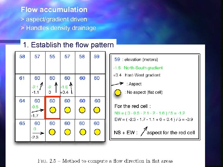Flow accumulation > aspect/gradient driven > Handles density drainage 1. Establish the flow pattern

2. Perform accumulation

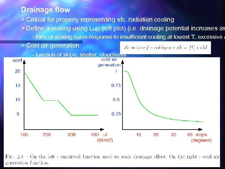Drainage flow > Critical for properly representing sfc. radiation cooling > Define a scaling using Lup (left plot) (i. e. drainage potential increases as - form of scaling curve response to insufficient cooling at lowest T, excessive a > Cold air generation - function of slope, shelter, cloudiness

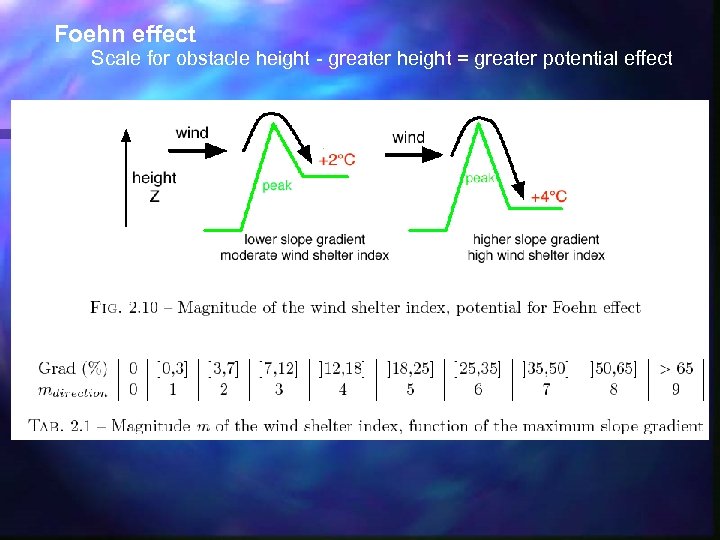Foehn effect Scale for obstacle height - greater height = greater potential effect

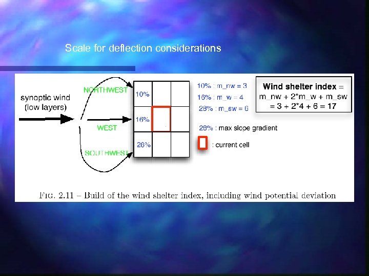Scale for deflection considerations

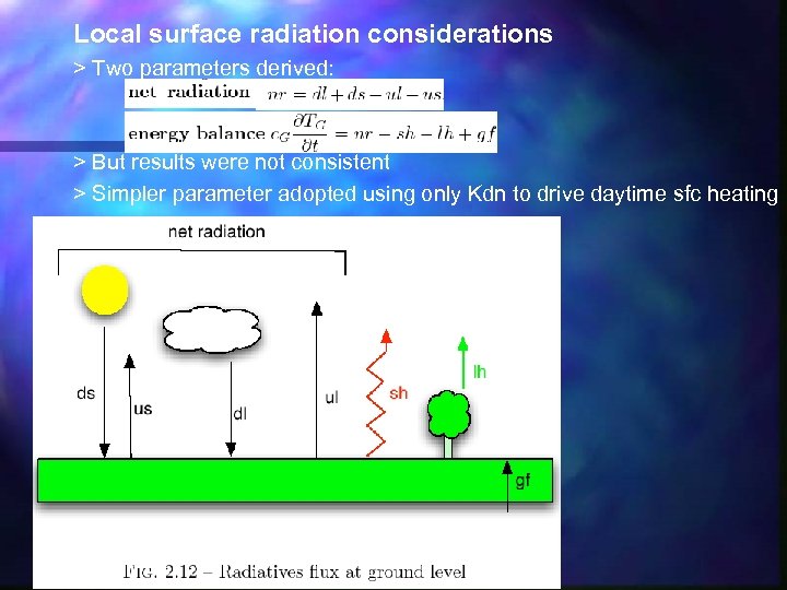Local surface radiation considerations > Two parameters derived: > But results were not consistent > Simpler parameter adopted using only Kdn to drive daytime sfc heating

Cold interior lowlands - drainage effect - captured Yukon Flats Central YK / Mackenzie valley

Impact of adding drainage, winds, adiabatic compression > 10 deg C diff in many areas

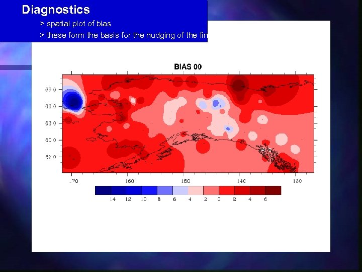Diagnostics > spatial plot of bias > these form the basis for the nudging of the final results

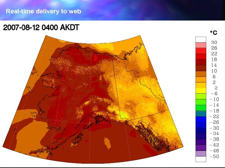Real-time delivery to web

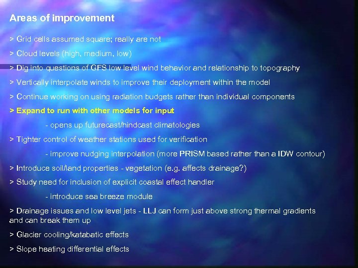Areas of improvement > Grid cells assumed square; really are not > Cloud levels (high, medium, low) > Dig into questions of GFS low level wind behavior and relationship to topography > Vertically interpolate winds to improve their deployment within the model > Continue working on using radiation budgets rather than individual components > Expand to run with other models for input - opens up futurecast/hindcast climatologies > Tighter control of weather stations used for verification - improve nudging interpolation (more PRISM based rather than a IDW contour) > Introduce soil/land properties - vegetation (e. g. affects drainage? ) > Study need for inclusion of explicit coastal effect handler - introduce sea breeze module > Drainage issues and low level jets - LLJ can form just above strong thermal gradients and can break them up > Glacier cooling/katabatic effects > Slope heating differential effects

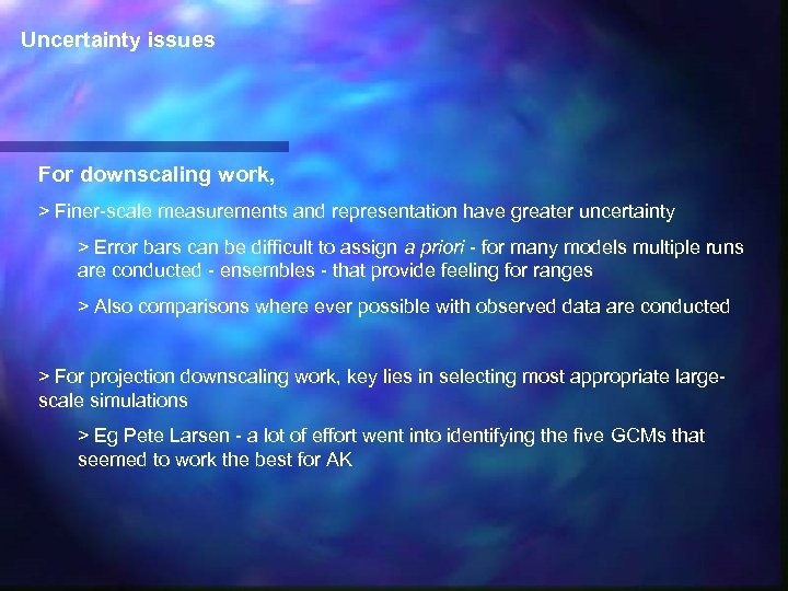Uncertainty issues For downscaling work, > Finer-scale measurements and representation have greater uncertainty > Error bars can be difficult to assign a priori - for many models multiple runs are conducted - ensembles - that provide feeling for ranges > Also comparisons where ever possible with observed data are conducted > For projection downscaling work, key lies in selecting most appropriate largescale simulations > Eg Pete Larsen - a lot of effort went into identifying the five GCMs that seemed to work the best for AK

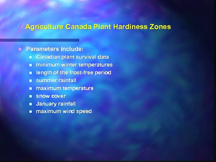Agriculture Canada Plant Hardiness Zones n Parameters include: n n n n Canadian plant survival data minimum winter temperatures length of the frost-free period summer rainfall maximum temperature snow cover January rainfall maximum wind speed

Topoclimate Model v 2. 0 (2007) Derived parameters (static) Slope gradient and aspect (8 directions) n Shelter/Exposure rating n n n A location behind a mountain range, for example, will be less exposed to cold air advection than a location on a plain Flow accumulation n Classic hydrology parameter but applies when density flows are a factor

Coastal effect > Built but not implemented > Coastal results worked fairly well without intervention

Shelter/Exposure determination > Determines extent to which cell affected by large-scale flow

Adiabatic compression/Foehn effect > Build mean wind vector over lowest layers (atm stability factored in w. Fr > Determine nature of exposure (shelter, obstacle wrt wind dir) > Scale for obstacle height - greater height = greater potential effect > Scale for deflection considerations

Results Results

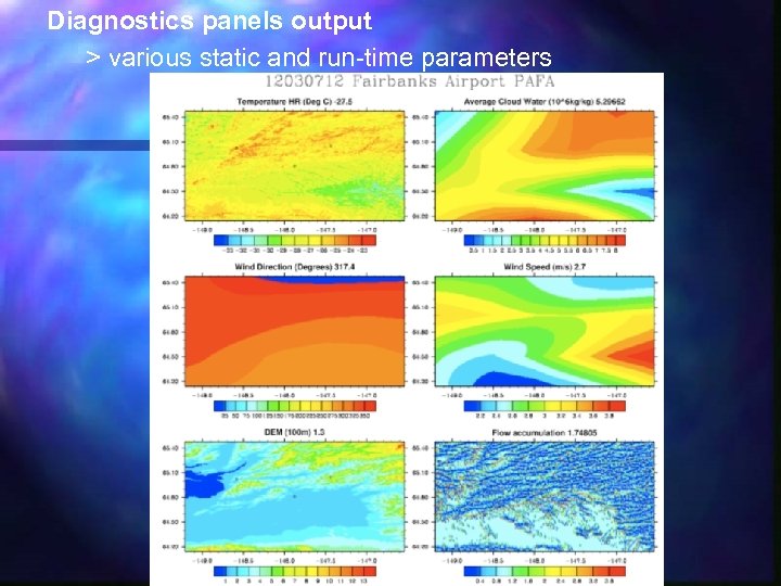Diagnostics panels output > various static and run-time parameters

Diagnostics panels output > radiation components

Diagnostics - biases > comparisons w. stations > 115 stns available Blue line= base est. Red line= all effects Average, April 2007: All stations

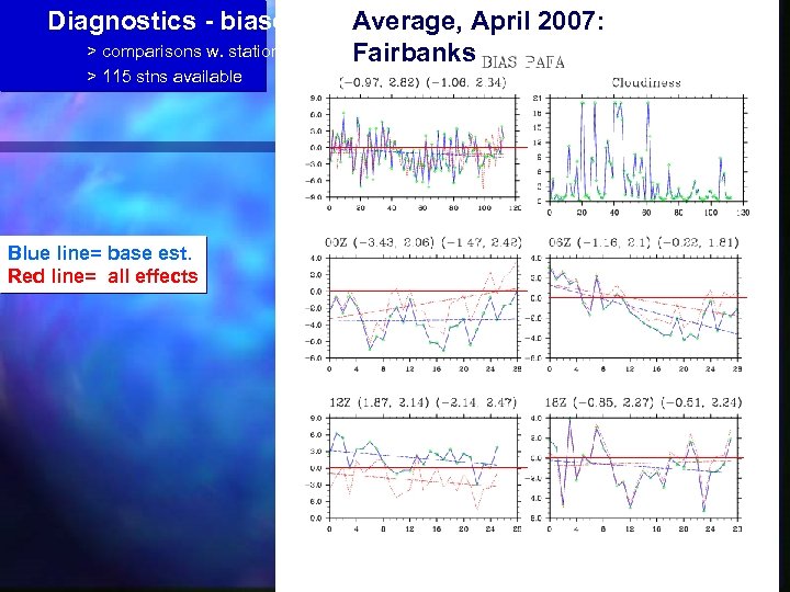Diagnostics - biases > comparisons w. stations > 115 stns available Blue line= base est. Red line= all effects Average, April 2007: Fairbanks

Diagnostics > comparisons w. stations > 115 stns available Blue line= base est. Red line= all effects Average, May 2007: All stations

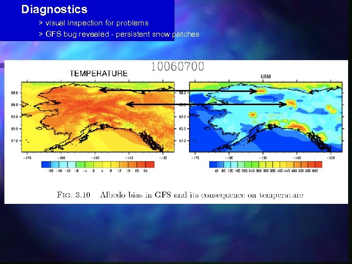Diagnostics > visual inspection for problems > GFS bug revealed - persistent snow patches