Empirical Methods for AI CS Paul Cohen

Empirical Methods for AI & CS Paul Cohen Ian P. Gent Toby Walsh cohen@cs. umass. edu ipg@dcs. st-and. ac. uk tw@cs. york. ac. uk

Overview z Introduction y What are empirical methods? y Why use them? z Case Study y Eight Basic Lessons z Experiment design z Data analysis z How not to do it z Supplementary material 2

Resources z Web www. cs. york. ac. uk/~tw/empirical. html www. cs. amherst. edu/~dsj/methday. html z Books “Empirical Methods for AI”, Paul Cohen, MIT Press, 1995 z Journals Journal of Experimental Algorithmics, www. jea. acm. org z Conferences Workshop on Empirical Methods in AI (last Saturday, ECAI-02? ) Workshop on Algorithm Engineering and Experiments, ALENEX 01 (alongside SODA) 3

Empirical Methods for CS Part I : Introduction

What does “empirical” mean? z Relying on observations, data, experiments z Empirical work should complement theoretical work y Theories often have holes (e. g. , How big is the constant term? Is the current problem a “bad” one? ) y Theories are suggested by observations y Theories are tested by observations y Conversely, theories direct our empirical attention z In addition (in this tutorial at least) empirical means “wanting to understand behavior of complex systems” 5

Why We Need Empirical Methods Cohen, 1990 Survey of 150 AAAI Papers z Roughly 60% of the papers gave no evidence that the work they described had been tried on more than a single example problem. z Roughly 80% of the papers made no attempt to explain performance, to tell us why it was good or bad and under which conditions it might be better or worse. z Only 16% of the papers offered anything that might be interpreted as a question or a hypothesis. z Theory papers generally had no applications or empirical work to support them, empirical papers were demonstrations, not experiments, and had no underlying theoretical support. z The essential synergy between theory and empirical work was missing 6

Theory, not Theorems z Theory based science need not be all theorems y otherwise science would be mathematics z Consider theory of QED y based on a model of behaviour of particles y predictions accurate to many decimal places (9? ) x most accurate theory in the whole of science? y success derived from accuracy of predictions x not the depth or difficulty or beauty of theorems y QED is an empirical theory! 7

Empirical CS/AI z Computer programs are formal objects y so let’s reason about them entirely formally? z Two reasons why we can’t or won’t: y theorems are hard y some questions are empirical in nature e. g. are Horn clauses adequate to represent the sort of knowledge met in practice? e. g. even though our problem is intractable in general, are the instances met in practice easy to solve? 8

Empirical CS/AI z Treat computer programs as natural objects y like fundamental particles, chemicals, living organisms z Build (approximate) theories about them y construct hypotheses e. g. greedy hill-climbing is important to GSAT y test with empirical experiments e. g. compare GSAT with other types of hill-climbing y refine hypotheses and modelling assumptions e. g. greediness not important, but hill-climbing is! 9

Empirical CS/AI z Many advantage over other sciences z Cost y no need for expensive super-colliders z Control y unlike the real world, we often have complete command of the experiment z Reproducibility y in theory, computers are entirely deterministic z Ethics y no ethics panels needed before you run experiments 10

Types of hypothesis z My search program is better than yours not very helpful beauty competition? z Search cost grows exponentially with number of variables for this kind of problem better as we can extrapolate to data not yet seen? z Constraint systems are better at handling over-constrained systems, but OR systems are better at handling underconstrained systems even better as we can extrapolate to new situations? 11

A typical conference conversation What are you up to these days? I’m running an experiment to compare the Davis-Putnam algorithm with GSAT? Why? I want to know which is faster Why? Lots of people use each of these algorithms How will these people use your result? . . . 12

Keep in mind the BIG picture What are you up to these days? I’m running an experiment to compare the Davis-Putnam algorithm with GSAT? Why? I have this hypothesis that neither will dominate What use is this? A portfolio containing both algorithms will be more robust than either algorithm on its own 13

Keep in mind the BIG picture. . . Why are you doing this? Because many real problems are intractable in theory but need to be solved in practice. How does your experiment help? It helps us understand the difference between average and worst case results So why is this interesting? Intractability is one of the BIG open questions in CS! 14

Why is empirical CS/AI in vogue? z Inadequacies of theoretical analysis y problems often aren’t as hard in practice as theory predicts in the worst-case y average-case analysis is very hard (and often based on questionable assumptions) z Some “spectacular” successes y phase transition behaviour y local search methods y theory lagging behind algorithm design 15

Why is empirical CS/AI in vogue? z Compute power ever increasing y even “intractable” problems coming into range y easy to perform large (and sometimes meaningful) experiments z Empirical CS/AI perceived to be “easier” than theoretical CS/AI y often a false perception as experiments easier to mess up than proofs 16

Empirical Methods for CS Part II: A Case Study Eight Basic Lessons

Rosenberg study z “An Empirical Study of Dynamic Scheduling on Rings of Processors” Gregory, Gao, Rosenberg & Cohen Proc. of 8 th IEEE Symp. on Parallel & Distributed Processing, 1996 Linked to from www. cs. york. ac. uk/~tw/empirical. html 18

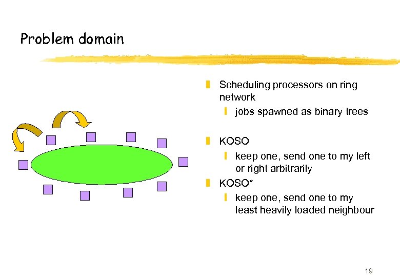Problem domain z Scheduling processors on ring network y jobs spawned as binary trees z KOSO y keep one, send one to my left or right arbitrarily z KOSO* y keep one, send one to my least heavily loaded neighbour 19

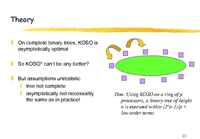Theory z On complete binary trees, KOSO is asymptotically optimal z So KOSO* can’t be any better? z But assumptions unrealistic y tree not complete y asymptotically not necessarily the same as in practice! Thm: Using KOSO on a ring of p processors, a binary tree of height n is executed within (2^n-1)/p + low order terms 20

Benefits of an empirical study z More realistic trees y probabilistic generator that makes shallow trees, which are “bushy” near root but quickly get “scrawny” y similar to trees generated when performing Trapezoid or Simpson’s Rule calculations x binary trees correspond to interval bisection z Startup costs y network must be loaded 21

Lesson 1: Evaluation begins with claims Lesson 2: Demonstration is good, understanding better z Hypothesis (or claim): KOSO takes longer than KOSO* because KOSO* balances loads better y The “because phrase” indicates a hypothesis about why it works. This is a better hypothesis than the beauty contest demonstration that KOSO* beats KOSO z Experiment design y Independent variables: KOSO v KOSO*, no. of processors, no. of jobs, probability(job will spawn), y Dependent variable: time to complete jobs 22

Criticism 1: This experiment design includes no direct measure of the hypothesized effect z Hypothesis: KOSO takes longer than KOSO* because KOSO* balances loads better z But experiment design includes no direct measure of load balancing: y Independent variables: KOSO v KOSO*, no. of processors, no. of jobs, probability(job will spawn), y Dependent variable: time to complete jobs 23

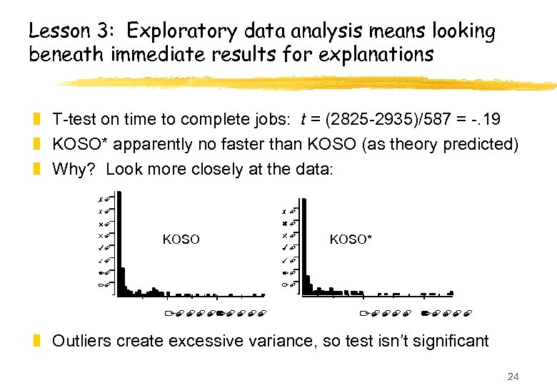Lesson 3: Exploratory data analysis means looking beneath immediate results for explanations z T-test on time to complete jobs: t = (2825 -2935)/587 = -. 19 z KOSO* apparently no faster than KOSO (as theory predicted) z Why? Look more closely at the data: 80 70 70 60 60 50 40 KOSO 50 40 30 30 20 20 10 KOSO* 10 1000020000 10000 20000 z Outliers create excessive variance, so test isn’t significant 24

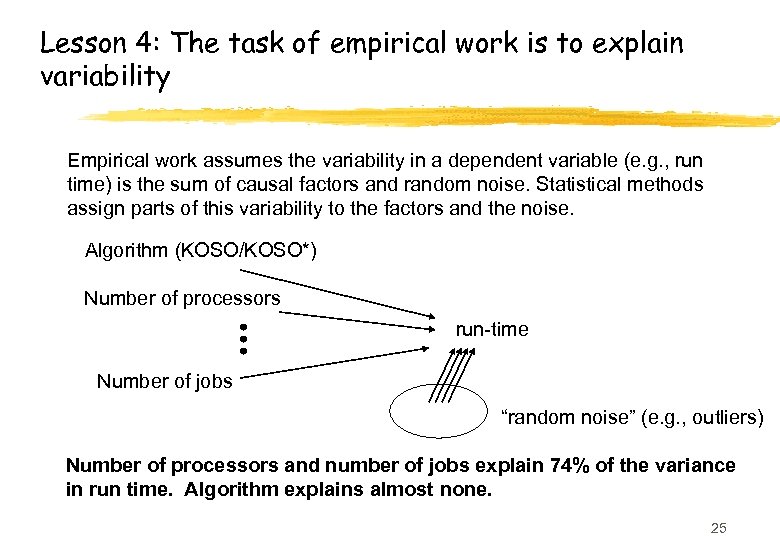Lesson 4: The task of empirical work is to explain variability Empirical work assumes the variability in a dependent variable (e. g. , run time) is the sum of causal factors and random noise. Statistical methods assign parts of this variability to the factors and the noise. Algorithm (KOSO/KOSO*) Number of processors run-time Number of jobs “random noise” (e. g. , outliers) Number of processors and number of jobs explain 74% of the variance in run time. Algorithm explains almost none. 25

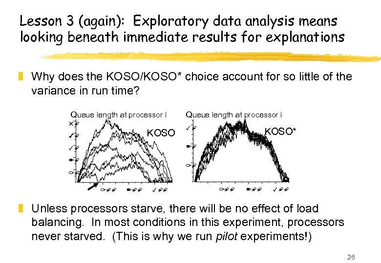Lesson 3 (again): Exploratory data analysis means looking beneath immediate results for explanations z Why does the KOSO/KOSO* choice account for so little of the variance in run time? Queue length at processor i 50 KOSO 40 Queue length at processor i 30 KOSO* 20 30 20 10 10 100 200 300 z Unless processors starve, there will be no effect of load balancing. In most conditions in this experiment, processors never starved. (This is why we run pilot experiments!) 26

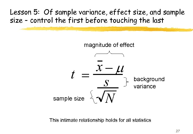Lesson 5: Of sample variance, effect size, and sample size – control the first before touching the last magnitude of effect x-m t = s sample size N background variance This intimate relationship holds for all statistics 27

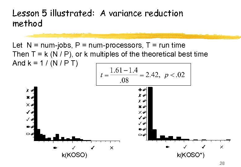Lesson 5 illustrated: A variance reduction method Let N = num-jobs, P = num-processors, T = run time Then T = k (N / P), or k multiples of theoretical best time And k = 1 / (N / P T) 90 80 70 60 50 40 30 20 10 2 3 k(KOSO) 4 5 2 3 4 5 k(KOSO*) 28

Where are we? z KOSO* is significantly better than KOSO when the dependent variable is recoded as percentage of optimal run time z The difference between KOSO* and KOSO explains very little of the variance in either dependent variable z Exploratory data analysis tells us that processors aren’t starving so we shouldn’t be surprised z Prediction: The effect of algorithm on run time (or k) increases as the number of jobs increases or the number of processors increases z This prediction is about interactions between factors 29

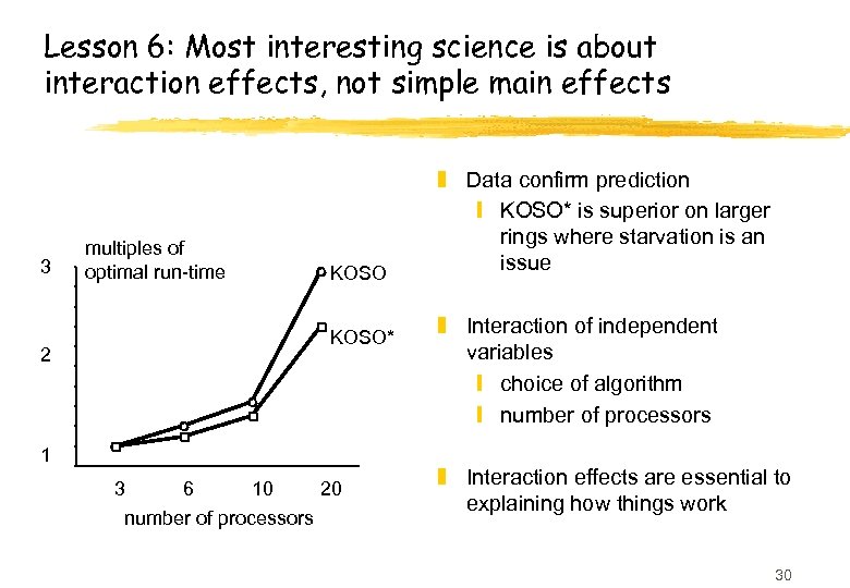Lesson 6: Most interesting science is about interaction effects, not simple main effects 3 2 multiples of optimal run-time KOSO* 1 3 6 10 20 number of processors z Data confirm prediction y KOSO* is superior on larger rings where starvation is an issue z Interaction of independent variables y choice of algorithm y number of processors z Interaction effects are essential to explaining how things work 30

Lesson 7: Significant and meaningful are not synonymous. Is a result meaningful? z KOSO* is significantly better than KOSO, but can you use the result? z Suppose you wanted to use the knowledge that the ring is controlled by KOSO or KOSO* for some prediction. y Grand median k = 1. 11; Pr(trial i has k > 1. 11) =. 5 y Pr(trial i under KOSO has k > 1. 11) = 0. 57 y Pr(trial i under KOSO* has k > 1. 11) = 0. 43 z Predict for trial i whether it’s k is above or below the median: y If it’s a KOSO* trial you’ll say no with (. 43 * 150) = 64. 5 errors y If it’s a KOSO trial you’ll say yes with ((1 -. 57) * 160) = 68. 8 errors y If you don’t know you’ll make (. 5 * 310) = 155 errors z 155 - (64. 5 + 68. 8) = 22 z Knowing the algorithm reduces error rate from. 5 to. 43. Is this enough? ? ? 31

Lesson 8: Keep the big picture in mind Why are you studying this? Load balancing is important to get good performance out of parallel computers Why is this important? Parallel computing promises to tackle many of our computational bottlenecks How do we know this? It’s in the first paragraph of the paper! 32

Case study: conclusions z Evaluation begins with claims z Demonstrations of simple main effects are good, understanding the effects is better z Exploratory data analysis means using your eyes to find explanatory patterns in data z The task of empirical work is to explain variablitity z Control variability before increasing sample size z Interaction effects are essential to explanations z Significant ≠ meaningful z Keep the big picture in mind 33

Empirical Methods for CS Part III : Experiment design

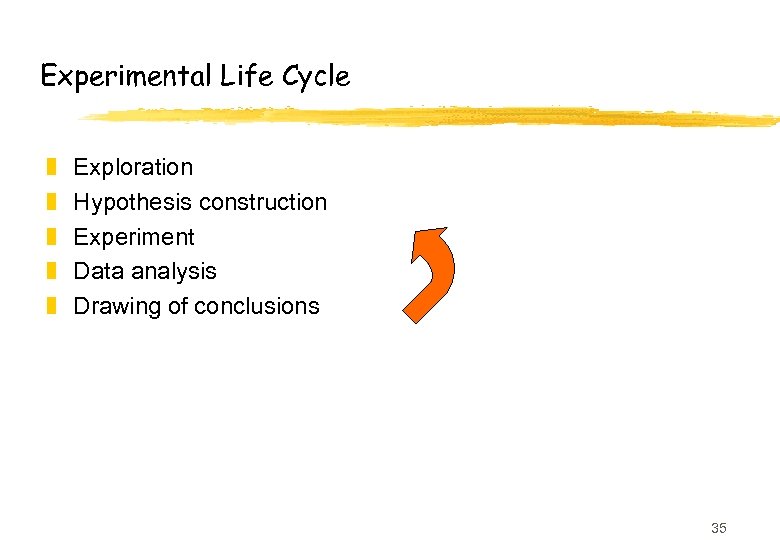Experimental Life Cycle z z z Exploration Hypothesis construction Experiment Data analysis Drawing of conclusions 35

Checklist for experiment design* z Consider the experimental procedure y making it explicit helps to identify spurious effects and sampling biases z Consider a sample data table y identifies what results need to be collected y clarifies dependent and independent variables y shows whether data pertain to hypothesis z Consider an example of the data analysis y helps you to avoid collecting too little or too much data y especially important when looking for interactions *From Chapter 3, “Empirical Methods for Artificial Intelligence”, Paul Cohen, MIT Press 36

Guidelines for experiment design z Consider possible results and their interpretation y may show that experiment cannot support/refute hypotheses under test y unforeseen outcomes may suggest new hypotheses z What was the question again? y easy to get carried away designing an experiment and lose the BIG picture z Run a pilot experiment to calibrate parameters (e. g. , number of processors in Rosenberg experiment) 37

Types of experiment z Manipulation experiment z Observation experiment z Factorial experiment 38

Manipulation experiment z Independent variable, x y x=identity of parser, size of dictionary, … z Dependent variable, y y y=accuracy, speed, … z Hypothesis y x influences y z Manipulation experiment y change x, record y 39

Observation experiment z Predictor, x y x=volatility of stock prices, … z Response variable, y y y=fund performance, … z Hypothesis y x influences y z Observation experiment y classify according to x, compute y 40

Factorial experiment z Several independent variables, xi y there may be no simple causal links y data may come that way e. g. individuals will have different sexes, ages, . . . z Factorial experiment y every possible combination of xi considered y expensive as its name suggests! 41

Designing factorial experiments z In general, stick to 2 to 3 independent variables z Solve same set of problems in each case y reduces variance due to differences between problem sets z If this not possible, use sample sizes y simplifies statistical analysis z As usual, default hypothesis is that no influence exists y much easier to fail to demonstrate influence than to demonstrate an influence 42

Some problem issues z Control z Ceiling and Floor effects z Sampling Biases 43

Control z A control is an experiment in which the hypothesised variation does not occur y so the hypothesized effect should not occur either z BUT remember y placebos cure a large percentage of patients! 44

Control: a cautionary tale z Macaque monkeys given vaccine based on human T-cells infected with SIV (relative of HIV) y macaques gained immunity from SIV z Later, macaques given uninfected human T-cells y and macaques still gained immunity! z Control experiment not originally done y and not always obvious (you can’t control for all variables) 45

Control: MYCIN case study z MYCIN was a medial expert system y recommended therapy for blood/meningitis infections z How to evaluate its recommendations? z Shortliffe used y 10 sample problems, 8 therapy recommenders x 5 faculty, 1 resident, 1 postdoc, 1 student y 8 impartial judges gave 1 point per problem y max score was 80 y Mycin 65, faculty 40 -60, postdoc 60, resident 45, student 30 46

Control: MYCIN case study z What were controls? z Control for judge’s bias for/against computers y judges did not know who recommended each therapy z Control for easy problems y medical student did badly, so problems not easy z Control for our standard being low y e. g. random choice should do worse z Control for factor of interest y e. g. hypothesis in MYCIN that “knowledge is power” y have groups with different levels of knowledge 47

Ceiling and Floor Effects z Well designed experiments (with good controls) can still go wrong z What if all our algorithms do particularly well y Or they all do badly? z We’ve got little evidence to choose between them 48

Ceiling and Floor Effects z Ceiling effects arise when test problems are insufficiently challenging y floor effects the opposite, when problems too challenging z A problem in AI because we often repeatedly use the same benchmark sets y most benchmarks will lose their challenge eventually? y but how do we detect this effect? 49

Machine learning example z 14 datasets from UCI corpus of benchmarks y used as mainstay of ML community z Problem is learning classification rules y each item is vector of features and a classification y measure classification accuracy of method (max 100%) z Compare C 4 with 1 R*, two competing algorithms Rob Holte, Machine Learning, vol. 3, pp. 63 -91, 1993 www. site. uottawa. edu/~holte/Publications/simple_rules. ps 50

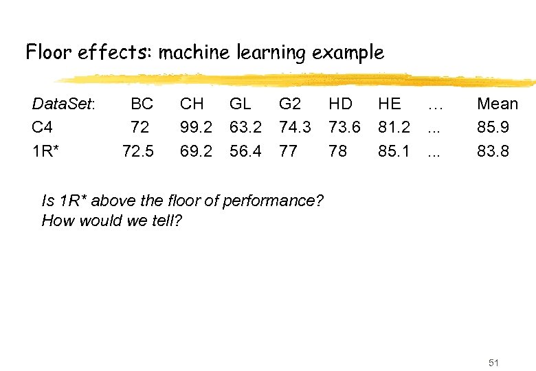Floor effects: machine learning example Data. Set: C 4 1 R* BC 72 72. 5 CH 99. 2 69. 2 GL 63. 2 56. 4 G 2 74. 3 77 HD 73. 6 78 HE 81. 2 85. 1 …. . . Mean 85. 9 83. 8 Is 1 R* above the floor of performance? How would we tell? 51

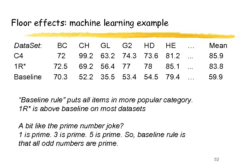Floor effects: machine learning example Data. Set: C 4 1 R* Baseline BC 72 72. 5 70. 3 CH 99. 2 69. 2 52. 2 GL 63. 2 56. 4 35. 5 G 2 74. 3 77 53. 4 HD 73. 6 78 54. 5 HE 81. 2 85. 1 79. 4 …. . . … Mean 85. 9 83. 8 59. 9 “Baseline rule” puts all items in more popular category. 1 R* is above baseline on most datasets A bit like the prime number joke? 1 is prime. 3 is prime. 5 is prime. So, baseline rule is that all odd numbers are prime. 52

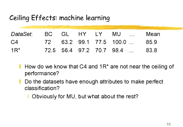Ceiling Effects: machine learning Data. Set: C 4 1 R* BC 72 72. 5 GL 63. 2 56. 4 HY 99. 1 97. 2 LY 77. 5 70. 7 MU … 100. 0. . . 98. 4. . . Mean 85. 9 83. 8 y How do we know that C 4 and 1 R* are not near the ceiling of performance? y Do the datasets have enough attributes to make perfect classification? x Obviously for MU, but what about the rest? 53

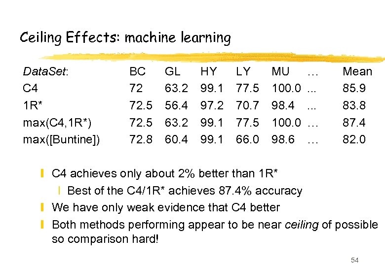Ceiling Effects: machine learning Data. Set: C 4 1 R* max(C 4, 1 R*) max([Buntine]) BC 72 72. 5 72. 8 GL 63. 2 56. 4 63. 2 60. 4 HY 99. 1 97. 2 99. 1 LY 77. 5 70. 7 77. 5 66. 0 MU 100. 0 98. 4 100. 0 98. 6 …. . . … … Mean 85. 9 83. 8 87. 4 82. 0 y C 4 achieves only about 2% better than 1 R* x Best of the C 4/1 R* achieves 87. 4% accuracy y We have only weak evidence that C 4 better y Both methods performing appear to be near ceiling of possible so comparison hard! 54

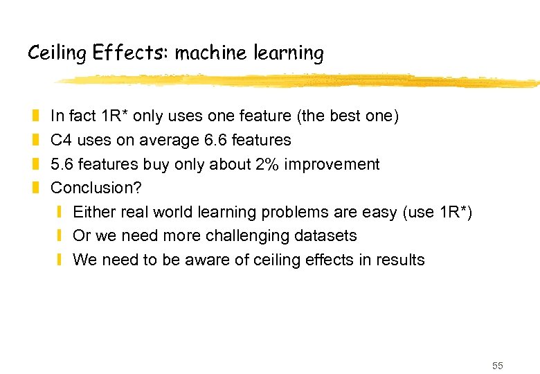Ceiling Effects: machine learning z z In fact 1 R* only uses one feature (the best one) C 4 uses on average 6. 6 features 5. 6 features buy only about 2% improvement Conclusion? y Either real world learning problems are easy (use 1 R*) y Or we need more challenging datasets y We need to be aware of ceiling effects in results 55

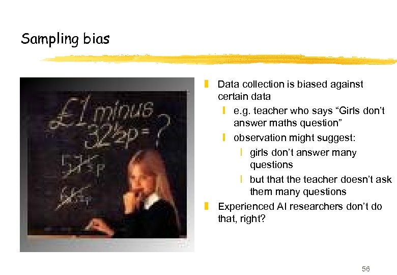Sampling bias z Data collection is biased against certain data y e. g. teacher who says “Girls don’t answer maths question” y observation might suggest: x girls don’t answer many questions x but that the teacher doesn’t ask them many questions z Experienced AI researchers don’t do that, right? 56

Sampling bias: Phoenix case study z AI system to fight (simulated) forest fires z Experiments suggest that wind speed uncorrelated with time to put out fire y obviously incorrect as high winds spread forest fires 57

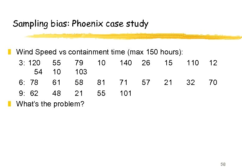Sampling bias: Phoenix case study z Wind Speed vs containment time (max 150 hours): 3: 120 55 79 10 140 26 15 110 54 10 103 6: 78 61 58 81 71 57 21 32 9: 62 48 21 55 101 z What’s the problem? 12 70 58

Sampling bias: Phoenix case study z The cut-off of 150 hours introduces sampling bias y many high-wind fires get cut off, not many low wind z On remaining data, there is no correlation between wind speed and time (r = -0. 53) z In fact, data shows that: y a lot of high wind fires take > 150 hours to contain y those that don’t are similar to low wind fires z You wouldn’t do this, right? y you might if you had automated data analysis. 59

Sampling biases can be subtle. . . z Assume gender (G) is an independent variable and number of siblings (S) is a noise variable. z If S is truly a noise variable then under random sampling, no dependency should exist between G and S in samples. z Parents have children until they get at least one boy. They don't feel the same way about girls. In a sample of 1000 girls the number with S = 0 is smaller than in a sample of 1000 boys. z The frequency distribution of S is different for different genders. S and G are not independent. z Girls do better at math than boys in random samples at all levels of education. z Is this because of their genes or because they have more siblings? z What else might be systematically associated with G that we don't know about? 60

Empirical Methods for CS Part IV: Data analysis

Kinds of data analysis z Exploratory (EDA) – looking for patterns in data z Statistical inferences from sample data y Testing hypotheses y Estimating parameters z Building mathematical models of datasets z Machine learning, data mining… z We will introduce hypothesis testing and computer-intensive methods 62

The logic of hypothesis testing z Example: toss a coin ten times, observe eight heads. Is the coin fair (i. e. , what is it’s long run behavior? ) and what is your residual uncertainty? z You say, “If the coin were fair, then eight or more heads is pretty unlikely, so I think the coin isn’t fair. ” z Like proof by contradiction: Assert the opposite (the coin is fair) show that the sample result (≥ 8 heads) has low probability p, reject the assertion, with residual uncertainty related to p. z Estimate p with a sampling distribution. 63

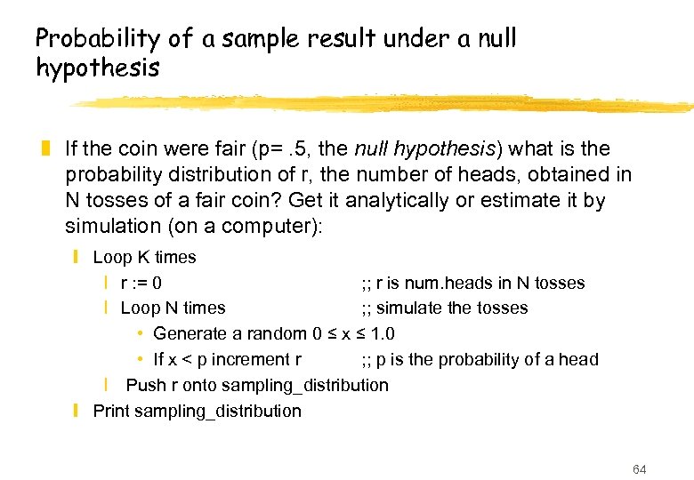Probability of a sample result under a null hypothesis z If the coin were fair (p=. 5, the null hypothesis) what is the probability distribution of r, the number of heads, obtained in N tosses of a fair coin? Get it analytically or estimate it by simulation (on a computer): y Loop K times x r : = 0 ; ; r is num. heads in N tosses x Loop N times ; ; simulate the tosses • Generate a random 0 ≤ x ≤ 1. 0 • If x < p increment r ; ; p is the probability of a head x Push r onto sampling_distribution y Print sampling_distribution 64

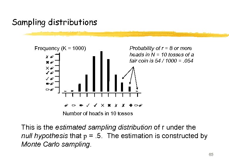Sampling distributions Frequency (K = 1000) 70 60 50 40 30 20 10 Probability of r = 8 or more heads in N = 10 tosses of a fair coin is 54 / 1000 =. 054 0 1 2 3 4 5 6 7 8 9 10 Number of heads in 10 tosses This is the estimated sampling distribution of r under the null hypothesis that p =. 5. The estimation is constructed by Monte Carlo sampling. 65

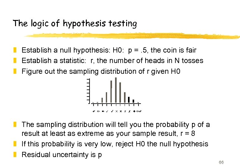The logic of hypothesis testing z Establish a null hypothesis: H 0: p =. 5, the coin is fair z Establish a statistic: r, the number of heads in N tosses z Figure out the sampling distribution of r given H 0 0 1 2 3 4 5 6 7 8 9 10 z The sampling distribution will tell you the probability p of a result at least as extreme as your sample result, r = 8 z If this probability is very low, reject H 0 the null hypothesis z Residual uncertainty is p 66

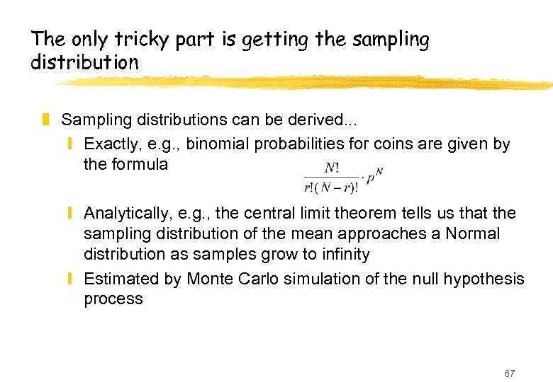The only tricky part is getting the sampling distribution z Sampling distributions can be derived. . . y Exactly, e. g. , binomial probabilities for coins are given by the formula y Analytically, e. g. , the central limit theorem tells us that the sampling distribution of the mean approaches a Normal distribution as samples grow to infinity y Estimated by Monte Carlo simulation of the null hypothesis process 67

A common statistical test: The Z test for different means z A sample N = 25 computer science students has mean IQ m=135. Are they “smarter than average”? z Population mean is 100 with standard deviation 15 z The null hypothesis, H 0, is that the CS students are “average”, i. e. , the mean IQ of the population of CS students is 100. z What is the probability p of drawing the sample if H 0 were true? If p small, then H 0 probably false. z Find the sampling distribution of the mean of a sample of size 25, from population with mean 100 68

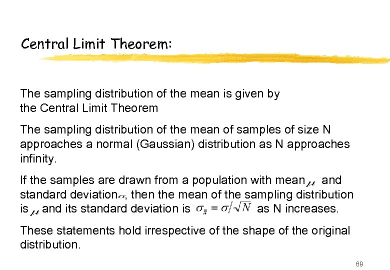Central Limit Theorem: The sampling distribution of the mean is given by the Central Limit Theorem The sampling distribution of the mean of samples of size N approaches a normal (Gaussian) distribution as N approaches infinity. If the samples are drawn from a population with mean and standard deviation , then the mean of the sampling distribution is and its standard deviation is as N increases. These statements hold irrespective of the shape of the original distribution. 69

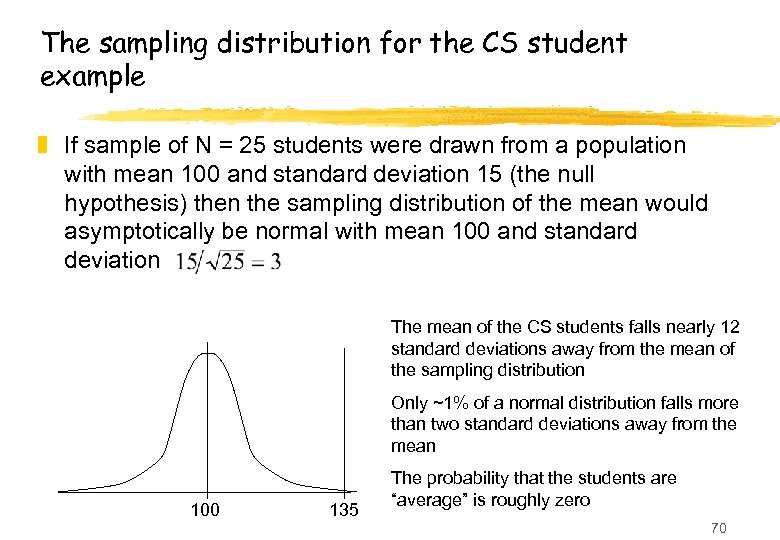The sampling distribution for the CS student example z If sample of N = 25 students were drawn from a population with mean 100 and standard deviation 15 (the null hypothesis) then the sampling distribution of the mean would asymptotically be normal with mean 100 and standard deviation The mean of the CS students falls nearly 12 standard deviations away from the mean of the sampling distribution Only ~1% of a normal distribution falls more than two standard deviations away from the mean 100 135 The probability that the students are “average” is roughly zero 70

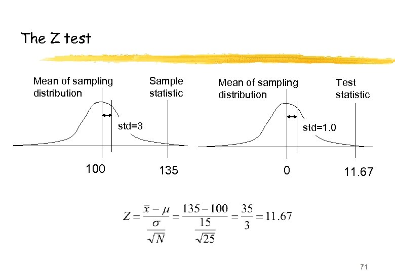The Z test Mean of sampling distribution Sample statistic Mean of sampling distribution std=3 100 Test statistic std=1. 0 135 0 11. 67 71

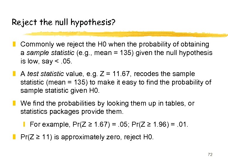Reject the null hypothesis? z Commonly we reject the H 0 when the probability of obtaining a sample statistic (e. g. , mean = 135) given the null hypothesis is low, say <. 05. z A test statistic value, e. g. Z = 11. 67, recodes the sample statistic (mean = 135) to make it easy to find the probability of sample statistic given H 0. z We find the probabilities by looking them up in tables, or statistics packages provide them. y For example, Pr(Z ≥ 1. 67) =. 05; Pr(Z ≥ 1. 96) =. 01. z Pr(Z ≥ 11) is approximately zero, reject H 0. 72

The t test z Same logic as the Z test, but appropriate when population standard deviation is unknown, samples are small, etc. z Sampling distribution is t, not normal, but approaches normal as samples size increases z Test statistic has very similar form but probabilities of the test statistic are obtained by consulting tables of the t distribution, not the normal 73

The t test Suppose N = 5 students have mean IQ = 135, std = 27 Estimate the standard deviation of sampling distribution using the sample standard deviation Mean of sampling distribution Sample statistic Mean of sampling distribution std=12. 1 100 135 Test statistic std=1. 0 0 2. 89 74

Summary of hypothesis testing z H 0 negates what you want to demonstrate; find probability p of sample statistic under H 0 by comparing test statistic to sampling distribution; if probability is low, reject H 0 with residual uncertainty proportional to p. z Example: Want to demonstrate that CS graduate students are smarter than average. H 0 is that they are average. t = 2. 89, p ≤. 022 z Have we proved CS students are smarter? NO! z We have only shown that mean = 135 is unlikely if they aren’t. We never prove what we want to demonstrate, we only reject H 0, with residual uncertainty. z And failing to reject H 0 does not prove H 0, either! 75

Common tests Tests that means are equal Tests that samples are uncorrelated or independent Tests that slopes of lines are equal Tests that predictors in rules have predictive power Tests that frequency distributions (how often events happen) are equal z Tests that classification variables such as smoking history and heart disease history are unrelated. . . z All follow the same basic logic z z z 76

Computer-intensive Methods z Basic idea: Construct sampling distributions by simulating on a computer the process of drawing samples. z Three main methods: y Monte carlo simulation when one knows population parameters; y Bootstrap when one doesn’t; y Randomization, also assumes nothing about the population. z Enormous advantage: Works for any statistic and makes no strong parametric assumptions (e. g. , normality) 77

Another Monte Carlo example, relevant to machine learning. . . z Suppose you want to buy stocks in a mutual fund; for simplicity assume there are just N = 50 funds to choose from and you’ll base your decision on the proportion of J=30 stocks in each fund that increased in value z Suppose Pr(a stock increasing in price) =. 75 z You are tempted by the best of the funds, F, which reports price increases in 28 of its 30 stocks. z What is the probability of this performance? 78

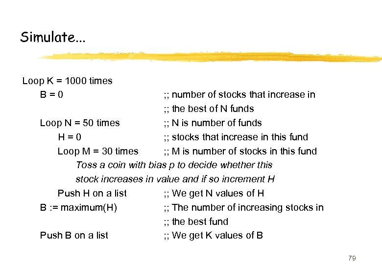Simulate. . . Loop K = 1000 times B=0 ; ; number of stocks that increase in ; ; the best of N funds Loop N = 50 times ; ; N is number of funds H=0 ; ; stocks that increase in this fund Loop M = 30 times ; ; M is number of stocks in this fund Toss a coin with bias p to decide whether this stock increases in value and if so increment H Push H on a list ; ; We get N values of H B : = maximum(H) ; ; The number of increasing stocks in ; ; the best fund Push B on a list ; ; We get K values of B 79

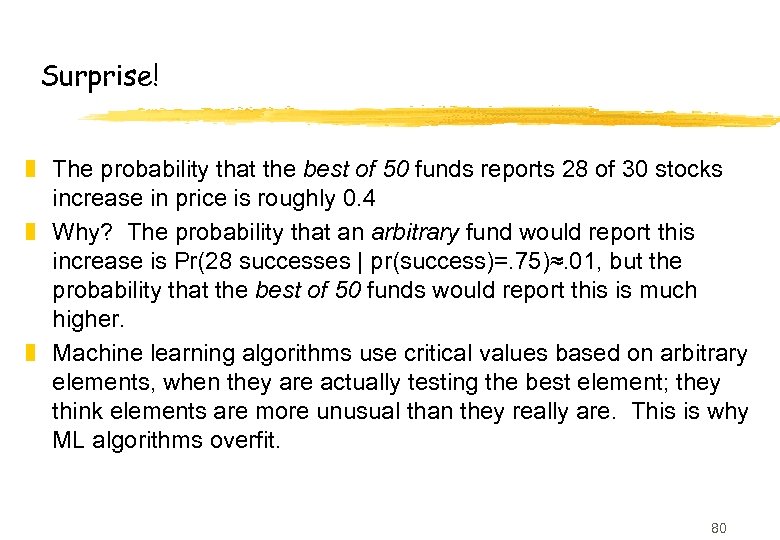Surprise! z The probability that the best of 50 funds reports 28 of 30 stocks increase in price is roughly 0. 4 z Why? The probability that an arbitrary fund would report this increase is Pr(28 successes | pr(success)=. 75)≈. 01, but the probability that the best of 50 funds would report this is much higher. z Machine learning algorithms use critical values based on arbitrary elements, when they are actually testing the best element; they think elements are more unusual than they really are. This is why ML algorithms overfit. 80

The Bootstrap z Monte Carlo estimation of sampling distributions assume you know the parameters of the population from which samples are drawn. z What if you don’t? z Use the sample as an estimate of the population. z Draw samples from the sample! z With or without replacement? z Example: Sampling distribution of the mean; check the results against the central limit theorem. 81

Bootstrapping the sampling distribution of the mean* z S is a sample of size N: Loop K = 1000 times Draw a pseudosample S* of size N from S by sampling with replacement Calculate the mean of S* and push it on a list L z L is the bootstrapped sampling distribution of the mean** z This procedure works for any statistic, not just the mean. * Recall we can get the sampling distribution of the mean via the central limit theorem – this example is just for illustration. ** This distribution is not a null hypothesis distribution and so is not directly used for hypothesis testing, but 82 can easily be transformed into a null hypothesis distribution (see Cohen, 1995).

Randomization z Used to test hypotheses that involve association between elements of two or more groups; very general. z Example: Paul tosses H H, Carole tosses T T is outcome independent of tosser? z Example: 4 women score 54 66 64 61, six men score 23 28 27 31 51 32. Is score independent of gender? z Basic procedure: Calculate a statistic f for your sample; randomize one factor relative to the other and calculate your pseudostatistic f*. Compare f to the sampling distribution for f*. 83

Example of randomization z Four women score 54 66 64 61, six men score 23 28 27 31 51 32. Is score independent of gender? z f = difference of means of men’s and women’s scores: 29. 25 z Under the null hypothesis of no association between gender and score, the score 54 might equally well have been achieved by a male or a female. z Toss all scores in a hopper, draw out four at random and without replacement, call them female*, call the rest male*, and calculate f*, the difference of means of female* and male*. Repeat to get a distribution of f*. This is an estimate of the sampling distribution of f under H 0: no difference between male and female scores. 84

Empirical Methods for CS Part V: How Not To Do It

Tales from the coal face z Those ignorant of history are doomed to repeat it y we have committed many howlers z We hope to help others avoid similar ones … … and illustrate how easy it is to screw up! z “How Not to Do It” I Gent, S A Grant, E. Mac. Intyre, P Prosser, P Shaw, B M Smith, and T Walsh University of Leeds Research Report, May 1997 z Every howler we report committed by at least one of the above authors! 86

How Not to Do It z Do measure with many instruments y in exploring hard problems, we used our best algorithms y missed very poor performance of less good algorithms better algorithms will be bitten by same effect on larger instances than we considered z Do measure CPU time y in exploratory code, CPU time often misleading y but can also be very informative e. g. heuristic needed more search but was faster 87

How Not to Do It z Do vary all relevant factors z Don’t change two things at once y ascribed effects of heuristic to the algorithm x changed heuristic and algorithm at the same time x didn’t perform factorial experiment y but it’s not always easy/possible to do the “right” experiments if there are many factors 88

How Not to Do It z Do Collect All Data Possible …. (within reason) y one year Santa Claus had to repeat all our experiments x ECAI/AAAI/IJCAI deadlines just after new year! y we had collected number of branches in search tree x performance scaled with backtracks, not branches x all experiments had to be rerun z Don’t Kill Your Machines y we have got into trouble with sysadmins … over experimental data we never used y often the vital experiment is small and quick 89

How Not to Do It z Do It All Again … (or at least be able to) y e. g. storing random seeds used in experiments y we didn’t do that and might have lost important result z Do Be Paranoid y “identical” implementations in C, Scheme gave different results z Do Use The Same Problems y reproducibility is a key to science (c. f. cold fusion) y can reduce variance 90

Choosing your test data z We’ve seen the possible problem of over-fitting y remember machine learning benchmarks? z Two common approaches y benchmark libraries y random problems z Both have potential pitfalls 91

Benchmark libraries z +ve y can be based on real problems y lots of structure z -ve y library of fixed size possible to over-fit algorithms to library y problems have fixed size so can’t measure scaling 92

Random problems z +ve y problems can have any size so can measure scaling y can generate any number of problems hard to over-fit? z -ve y may not be representative of real problems x lack structure y easy to generate “flawed” problems x CSP, QSAT, … 93

Flawed random problems z Constraint satisfaction example y 40+ papers over 5 years by many authors used Models A, B, C, and D y all four models are “flawed” [Achlioptas et al. 1997] x asymptotically almost all problems are trivial x brings into doubt many experimental results • some experiments at typical sizes affected • fortunately not many y How should we generate problems in future? 94

Flawed random problems z [Gent et al. 1998] fix flaw …. y introduce “flawless” problem generation y defined in two equivalent ways y though no proof that problems are truly flawless z Undergraduate student at Strathclyde found new bug y two definitions of flawless not equivalent z Eventually settled on final definition of flawless y gave proof of asymptotic non-triviality y so we think that we just about understand the problem generator now 95

Prototyping your algorithm z Often need to implement an algorithm y usually novel algorithm, or variant of existing one x e. g. new heuristic in existing search algorithm y novelty of algorithm should imply extra care y more often, encourages lax implementation x it’s only a preliminary version 96

How Not to Do It z Don’t Trust Yourself y bug in innermost loop found by chance y all experiments re-run with urgent deadline y curiously, sometimes bugged version was better! z Do Preserve Your Code y Or end up fixing the same error twice Do use version control! 97

How Not to Do It z Do Make it Fast Enough y emphasis on enough x it’s often not necessary to have optimal code x in lifecycle of experiment, extra coding time not won back y e. g. we have published many papers with inefficient code x compared to state of the art • first GSAT version O(N 2), but this really was too slow! • Do Report Important Implementation Details x Intermediate versions produced good results 98

How Not to Do It z Do Look at the Raw Data y Summaries obscure important aspects of behaviour y Many statistical measures explicitly designed to minimise effect of outliers y Sometimes outliers are vital x “exceptionally hard problems” dominate mean x we missed them until they hit us on the head when experiments “crashed” overnight old data on smaller problems showed clear behaviour 99

How Not to Do It z Do face up to the consequences of your results y e. g. preprocessing on 450 problems x should “obviously” reduce search x reduced search 448 times x increased search 2 times y Forget algorithm, it’s useless? y Or study in detail the two exceptional cases x and achieve new understanding of an important algorithm 100

Empirical Methods for CS Part VII : Coda

Our objectives z Outline some of the basic issues y exploration, experimental design, data analysis, . . . z Encourage you to consider some of the pitfalls y we have fallen into all of them! z Raise standards y encouraging debate y identifying “best practice” z Learn from your experiences y experimenters get better as they get older! 102

Summary z Empirical CS and AI are exacting sciences y There are many ways to do experiments wrong z We are experts in doing experiments badly z As you perform experiments, you’ll make many mistakes z Learn from those mistakes, and ours! 103

Empirical Methods for CS Part VII : Supplement

Some expert advice z Bernard Moret, U. New Mexico “Towards a Discipline of Experimental Algorithmics” z David Johnson, AT&T Labs “A Theoretician’s Guide to the Experimental Analysis of Algorithms” Both linked to from www. cs. york. ac. uk/~tw/empirical. html 105

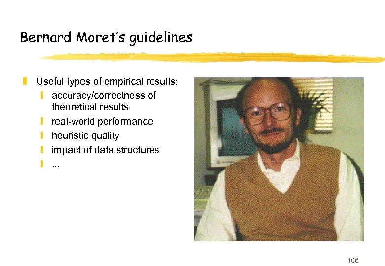Bernard Moret’s guidelines z Useful types of empirical results: y accuracy/correctness of theoretical results y real-world performance y heuristic quality y impact of data structures y. . . 106

Bernard Moret’s guidelines z Hallmarks of a good experimental paper y clearly defined goals y large scale tests both in number and size of instances y mixture of problems real-world, random, standard benchmarks, . . . y statistical analysis of results y reproducibility publicly available instances, code, data files, . . . 107

Bernard Moret’s guidelines z Pitfalls for experimental papers y simpler experiment would have given same result y result predictable by (back of the envelope) calculation y bad experimental setup e. g. insufficient sample size, no consideration of scaling, … y poor presentation of data e. g. lack of statistics, discarding of outliers, . . . 108

Bernard Moret’s guidelines z Ideal experimental procedure y define clear set of objectives which questions are you asking? y design experiments to meet these objectives y collect data do not change experiments until all data is collected to prevent drift/bias y analyse data consider new experiments in light of these results 109

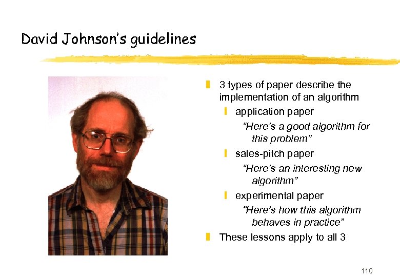David Johnson’s guidelines z 3 types of paper describe the implementation of an algorithm y application paper “Here’s a good algorithm for this problem” y sales-pitch paper “Here’s an interesting new algorithm” y experimental paper “Here’s how this algorithm behaves in practice” z These lessons apply to all 3 110

David Johnson’s guidelines z Perform “newsworthy” experiments y standards higher than for theoretical papers! y run experiments on real problems theoreticians can get away with idealized distributions but experimentalists have no excuse! y don’t use algorithms that theory can already dismiss y look for generality and relevance don’t just report algorithm A dominates algorithm B, identify why it does! 111

David Johnson’s guidelines z Place work in context y compare against previous work in literature y ideally, obtain their code and test sets verify their results, and compare with your new algorithm y less ideally, re-implement their code report any differences in performance y least ideally, simply report their old results try to make some ball-park comparisons of machine speeds 112

David Johnson’s guidelines z Use efficient implementations y “somewhat” controversial y efficient implementation supports claims of practicality tells us what is achievable in practice y can run more experiments on larger instances can do our research quicker! y don’t have to go over-board on this y exceptions can also be made e. g. not studying CPU time, comparing against a previously newsworthy algorithm, programming time more valuable than processing time, . . . 113

David Johnson’s guidelines z Use testbeds that support general conclusions y ideally one (or more) random class, & real world instances predict performance on real world problems based on random class, evaluate quality of predictions y structured random generators parameters to control structure as well as size y don’t just study real world instances hard to justify generality unless you have a very broad class of real world problems! 114

David Johnson’s guidelines z Provide explanations and back them up with experiment y adds to credibility of experimental results y improves our understanding of algorithms leading to better theory and algorithms y can “weed” out bugs in your implementation! 115

David Johnson’s guidelines z Ensure reproducibilty y easily achieved via the Web y adds support to a paper if others can (and do) reproduce the results y requires you to use large samples and wide range of problems otherwise results will not be reproducible! 116

David Johnson’s guidelines z Ensure comparability (and give the full picture) y make it easy for those who come after to reproduce your results y provide meaningful summaries give sample sizes, report standard deviations, plot graphs but report data in tables in the appendix y do not hide anomalous results y report running times even if this is not the main focus readers may want to know before studying your results in detail 117

David Johnson’s pitfalls z z z z Failing to report key implementation details Extrapolating from tiny samples Using irreproducible benchmarks Using running time as a stopping criterion Ignoring hidden costs (e. g. preprocessing) Misusing statistical tools Failing to use graphs 118

David Johnson’s pitfalls z z z Obscuring raw data by using hard-to-read charts Comparing apples and oranges Drawing conclusions not supported by the data Leaving obvious anomalies unnoted/unexplained Failing to back up explanations with further experiments Ignoring the literature the self-referential study! 119