Elasticity percentage for each hundred one per

Elasticity

percentage: “for each hundred” one per cent: one for each hundred ex: "I spend ten percent of my income on entertainment" means that "I spend ten dollars of each hundred dollars of my income on entertainment. "

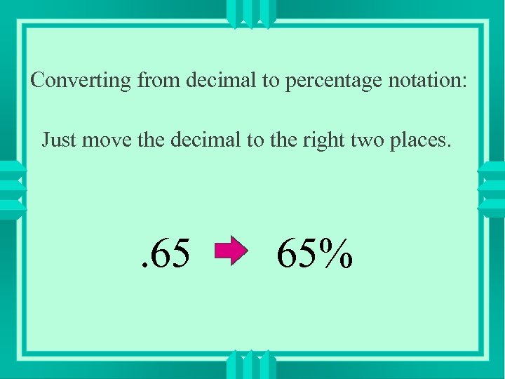Converting from decimal to percentage notation: Just move the decimal to the right two places. . 65 65%

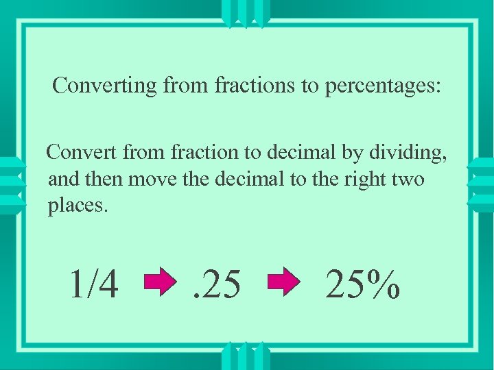Converting from fractions to percentages: Convert from fraction to decimal by dividing, and then move the decimal to the right two places. 1/4 . 25 25%

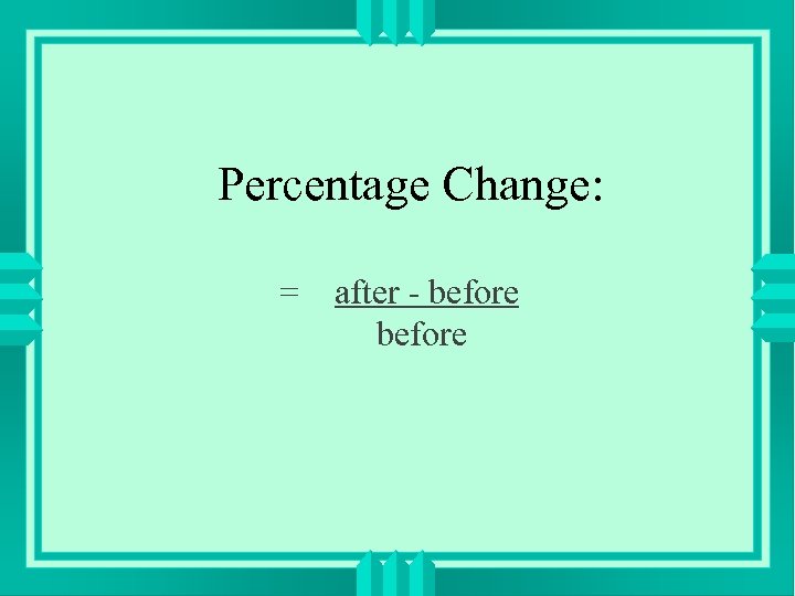Percentage Change: = after - before

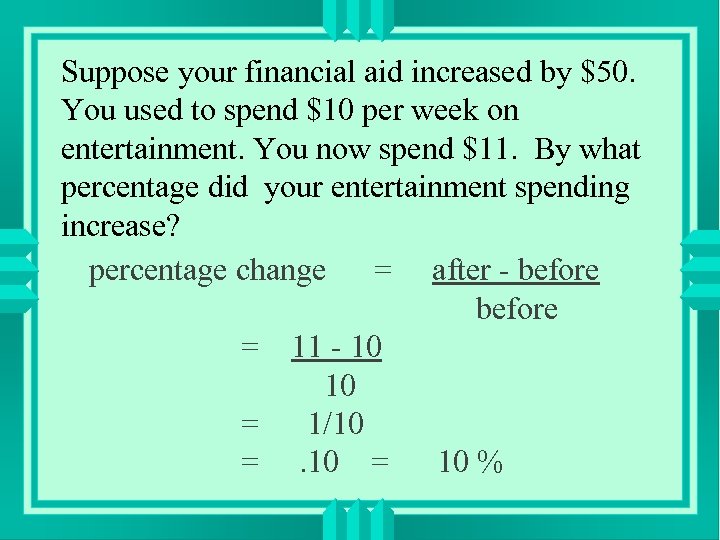Suppose your financial aid increased by $50. You used to spend $10 per week on entertainment. You now spend $11. By what percentage did your entertainment spending increase? percentage change = after - before = 11 - 10 10 = 1/10 = 10 %

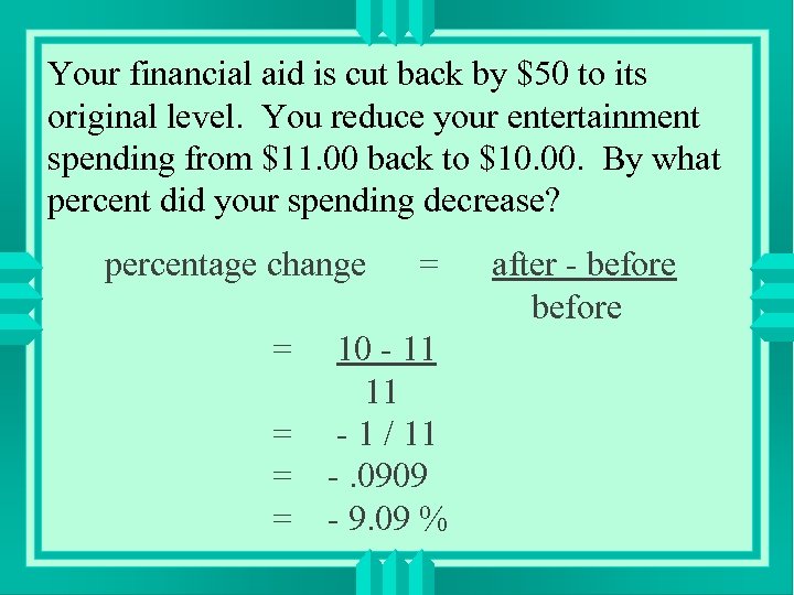Your financial aid is cut back by $50 to its original level. You reduce your entertainment spending from $11. 00 back to $10. 00. By what percent did your spending decrease? percentage change = = = 10 - 11 11 - 1 / 11 -. 0909 - 9. 09 % after - before

A negative change indicates a decrease. A positive change indicates an increase.

It would be nice to be able to say the following: In response to a $50 increase, you increased your spending by some percent x. In response to a $50 decrease, you decreased your spending by that same x percent. When we get to the concept of elasticity, in particular, we will want to be able to do that.

So we will define percentage changes a little differently. Instead of using our "before" value as our denominator, we will use the average (or midpoint) of our "before" and "after" values as the denominator. average = (before + after) / 2

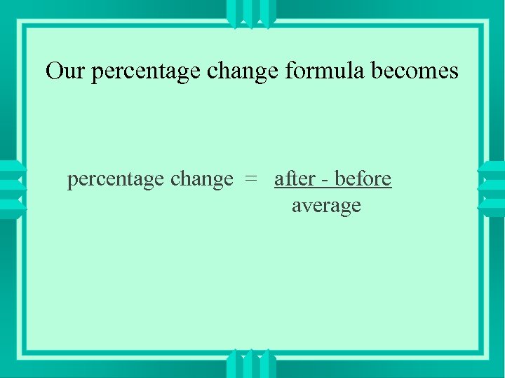Our percentage change formula becomes percentage change = after - before average

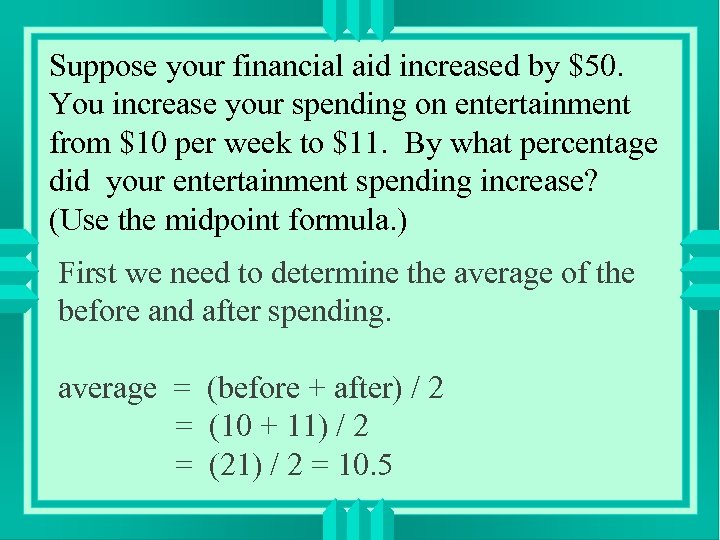Suppose your financial aid increased by $50. You increase your spending on entertainment from $10 per week to $11. By what percentage did your entertainment spending increase? (Use the midpoint formula. ) First we need to determine the average of the before and after spending. average = (before + after) / 2 = (10 + 11) / 2 = (21) / 2 = 10. 5

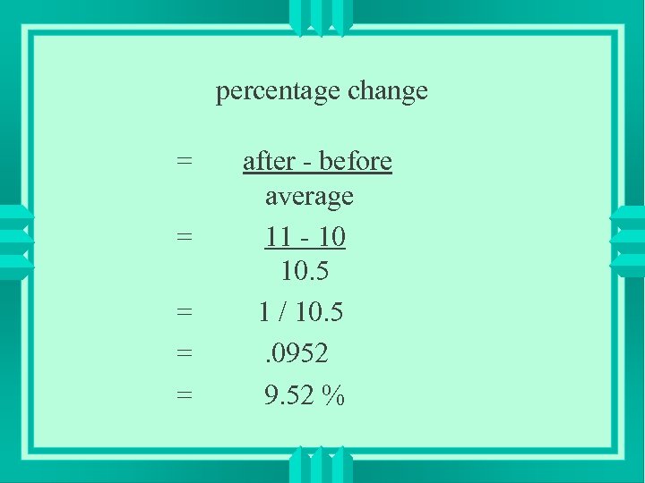percentage change = = = after - before average 11 - 10 10. 5 1 / 10. 5. 0952 9. 52 %

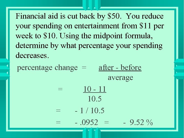Financial aid is cut back by $50. You reduce your spending on entertainment from $11 per week to $10. Using the midpoint formula, determine by what percentage your spending decreases. percentage change = after - before average = 10 - 11 10. 5 = - 1 / 10. 5 = -. 0952 = - 9. 52 %

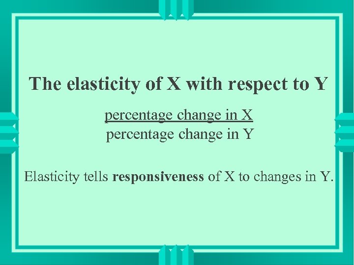The elasticity of X with respect to Y percentage change in X percentage change in Y Elasticity tells responsiveness of X to changes in Y.

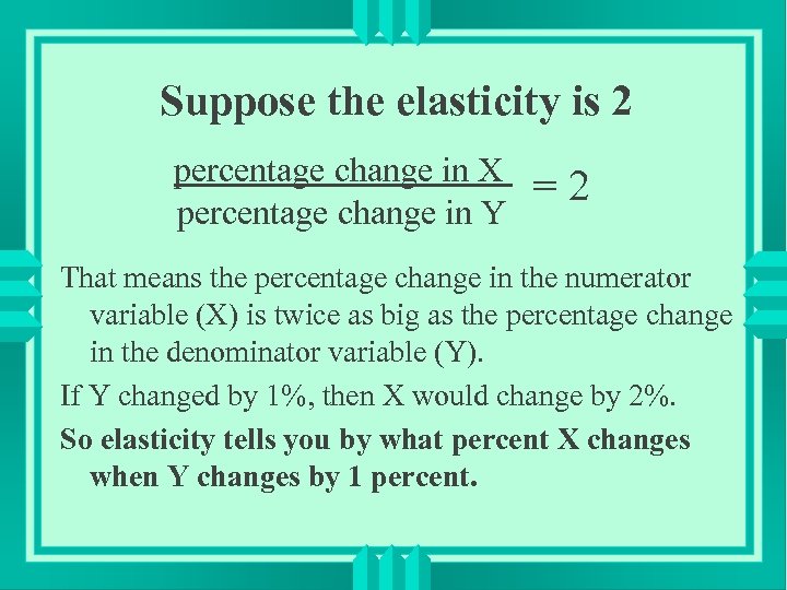Suppose the elasticity is 2 percentage change in X percentage change in Y =2 That means the percentage change in the numerator variable (X) is twice as big as the percentage change in the denominator variable (Y). If Y changed by 1%, then X would change by 2%. So elasticity tells you by what percent X changes when Y changes by 1 percent.

In the elasticity formula, how do you remember which variable goes on top and which goes underneath? u The cause goes under the line. CAUSE and UNDER both have a U. u The effect goes on top. EFFECT and TOP both have a T.

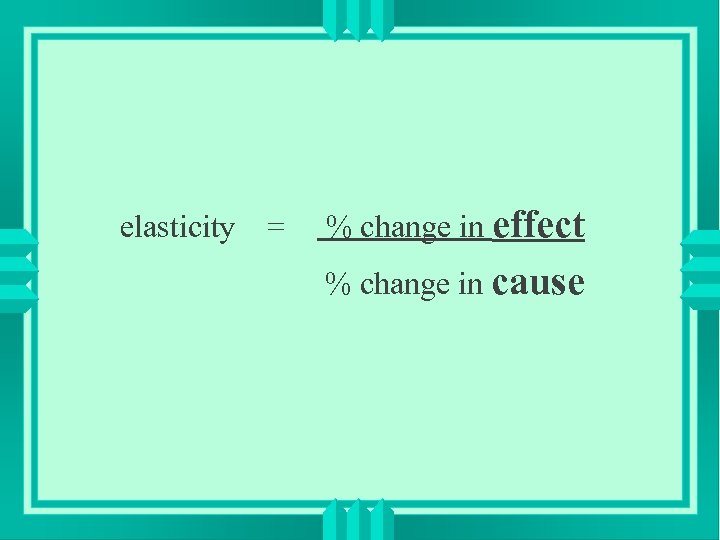elasticity = % change in effect % change in cause

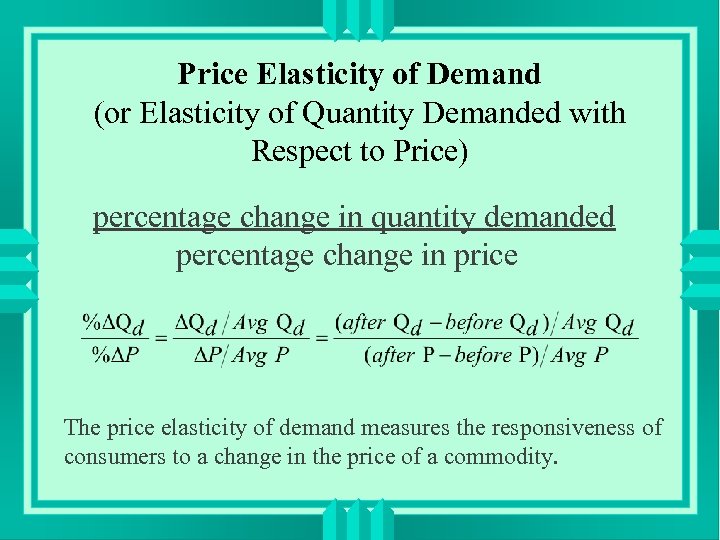Price Elasticity of Demand (or Elasticity of Quantity Demanded with Respect to Price) percentage change in quantity demanded percentage change in price The price elasticity of demand measures the responsiveness of consumers to a change in the price of a commodity.

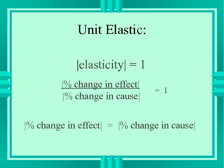Unit Elastic: |elasticity| = 1 |% change in effect| |% change in cause| = 1 |% change in effect| = |% change in cause|

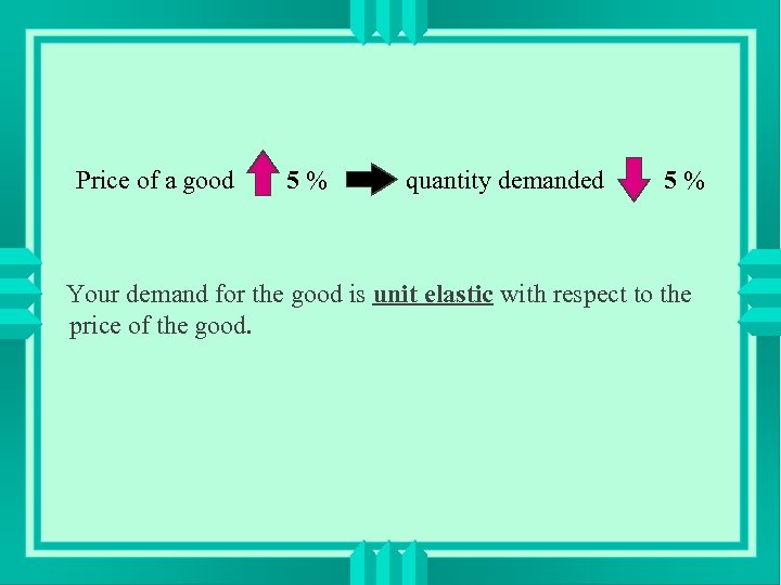Price of a good 5% quantity demanded 5% Your demand for the good is unit elastic with respect to the price of the good.

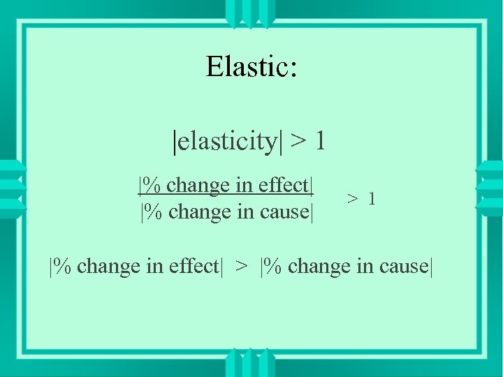Elastic: |elasticity| > 1 |% change in effect| |% change in cause| > 1 |% change in effect| > |% change in cause|

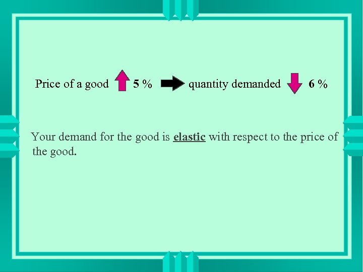Price of a good 5% quantity demanded 6% Your demand for the good is elastic with respect to the price of the good.

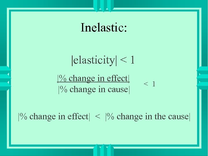Inelastic: |elasticity| < 1 |% change in effect| |% change in cause| < 1 |% change in effect| < |% change in the cause|

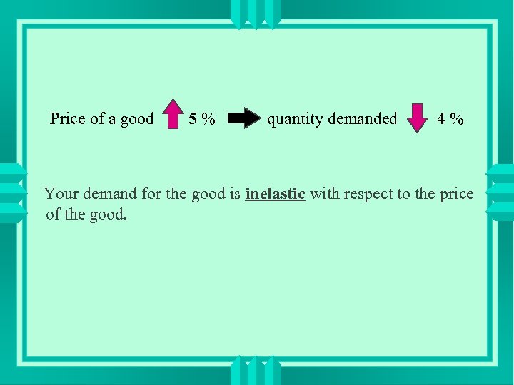Price of a good 5% quantity demanded 4% Your demand for the good is inelastic with respect to the price of the good.

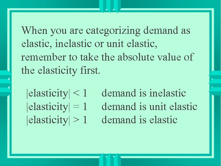When you are categorizing demand as elastic, inelastic or unit elastic, remember to take the absolute value of the elasticity first. |elasticity| < 1 |elasticity| = 1 |elasticity| > 1 demand is inelastic demand is unit elastic demand is elastic

Suppose the price of personal computers increased from $1600 to $1700. As a result, the number of PCs purchased per week by area consumers dropped from 500 to 400. Calculate the following: u the percentage change in the quantity demanded of PCs, u the percentage change in the price of PCs, and u the elasticity of demand for PCs with respect to the price of PCs.

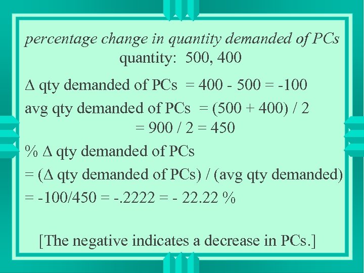percentage change in quantity demanded of PCs quantity: 500, 400 qty demanded of PCs = 400 - 500 = -100 avg qty demanded of PCs = (500 + 400) / 2 = 900 / 2 = 450 % qty demanded of PCs = ( qty demanded of PCs) / (avg qty demanded) = -100/450 = -. 2222 = - 22. 22 % [The negative indicates a decrease in PCs. ]

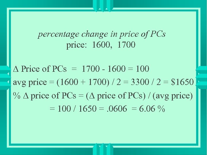percentage change in price of PCs price: 1600, 1700 Price of PCs = 1700 - 1600 = 100 avg price = (1600 + 1700) / 2 = 3300 / 2 = $1650 % price of PCs = ( price of PCs) / (avg price) = 100 / 1650 =. 0606 = 6. 06 %

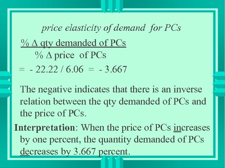price elasticity of demand for PCs % qty demanded of PCs % price of PCs = - 22. 22 / 6. 06 = - 3. 667 The negative indicates that there is an inverse relation between the qty demanded of PCs and the price of PCs. Interpretation: When the price of PCs increases by one percent, the quantity demanded of PCs decreases by 3. 667 percent.

|-3. 667| = 3. 667 > 1 So, the demand for PCs is elastic with respect to the price of PCs.

Because it is almost always the case that the qty demanded of a good is inversely related to its price, the negative sign is frequently dropped. ex: The price elasticity of demand for PCs would be reported as 3. 667 instead of -3. 667. The negative is understood.

Suppose you have an ailment, for which you must take a particular medication. (Call it Medex. ) Every Medex thirty days you purchase one thirtycapsule bottle of Medex. The price of Medex increases from $4 to $5 per bottle. You still purchase one bottle every thirty days. Calculate the elasticity of your quantity demanded of Medex with respect to the price of Medex.

price elasticity of demand for Medex % qty demanded of Medex % price of Medex = 0 because the numerator is zero (since the quantity demanded didn’t change) and the denominator is not zero (since the price did change).

Perfectly Inelasticity = 0 It is a special case of inelastic.

Suppose you are in the pizza business. As a very small company, you take the area price of pizza ($8) as given. That is, you always charge the same price. The quantity demanded of your pizza fluctuates. Last week, the quantity demanded of your pizza increased from 750 to 800 pizzas. Calculate the price elasticity of demand for your pizza.

price elasticity of demand for pizza % qty demanded of pizza % price of pizza = infinity or undefined because the denominator is zero (since the price didn’t change) and the numerator is not zero (since the quantity demanded did change).

Perfectly Elastic or Infinitely Elastic elasticity = infinity It is a special case of elastic.

Determinants of Price Elasticity of Demand 1. Elasticity of demand is greater if there are good substitutes available. Example: The elasticity of demand for a particular brand of gas would be quite high because there are lots of other brands of gas available.

Determinants of Price Elasticity of Demand 2. Elasticity of demand is greater if the price of the good is high relative to one’s budget. Example: The elasticity of demand for a salt is low because salt is a very small part of one’s budget.

Determinants of Price Elasticity of Demand 3. Elasticity of demand is greater if the product is a luxury rather than a necessity. Example: The elasticity of demand for insulin by a diabetic is extremely low because insulin is a necessity.

Determinants of Price Elasticity of Demand 4. Elasticity of demand is greater if the buyer has more time to adjust to a change in price. Example: The elasticity of demand for gas is more elastic when you allow people more time to adjust. If the price of gas goes up today, you can adjust your consumption only a little bit tomorrow. But if you have a few years, you can replace your car with one that consumes less gas and you can move closer to where you work.

Elasticity Graphs

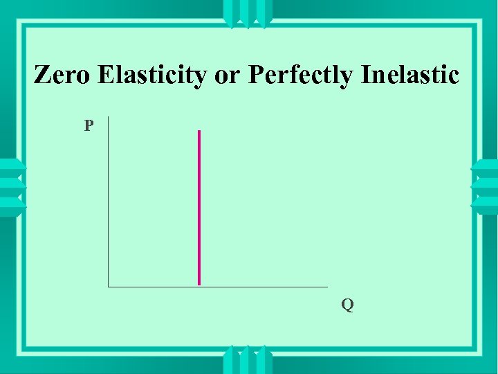Zero Elasticity or Perfectly Inelastic P Q

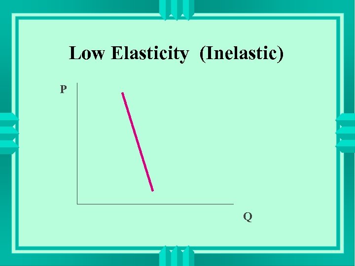Low Elasticity (Inelastic) P Q

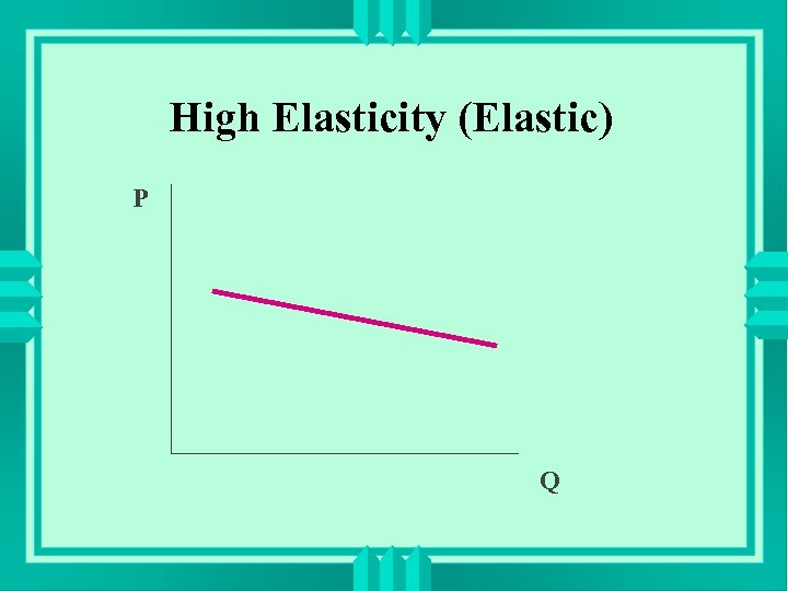High Elasticity (Elastic) P Q

Infinite Elasticity or Perfectly Elastic P Q

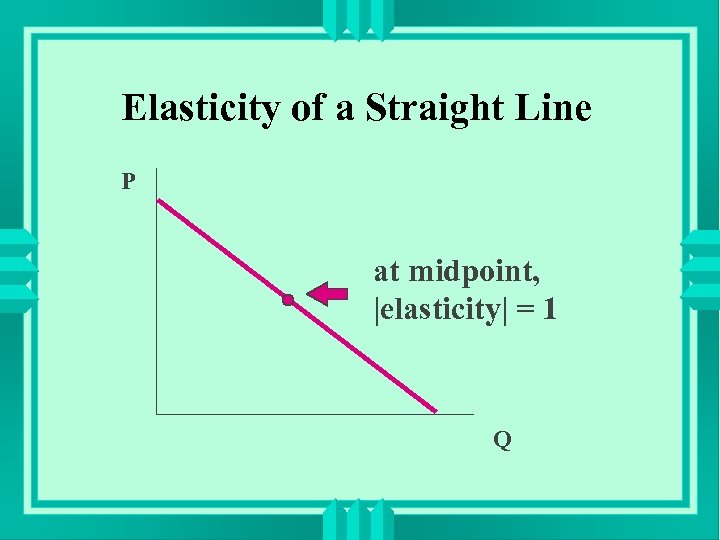Elasticity of a Straight Line P at midpoint, |elasticity| = 1 Q

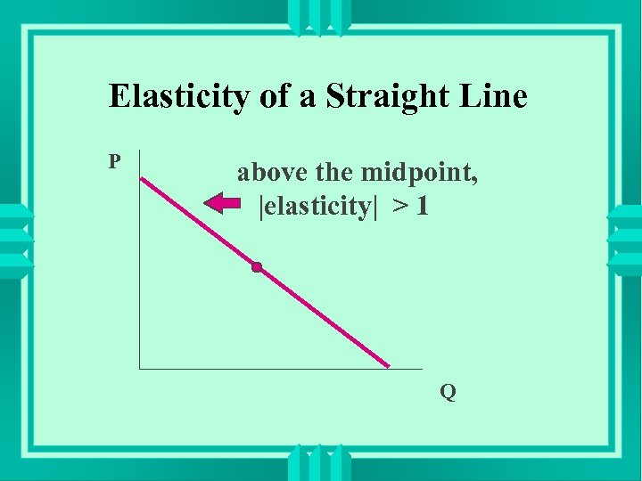Elasticity of a Straight Line P above the midpoint, |elasticity| > 1 Q

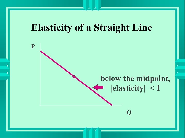Elasticity of a Straight Line P below the midpoint, |elasticity| < 1 Q

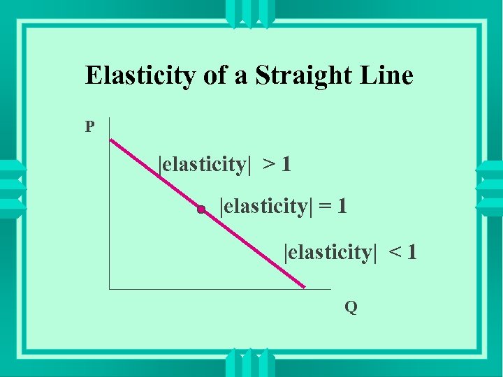Elasticity of a Straight Line P |elasticity| > 1 |elasticity| = 1 |elasticity| < 1 Q

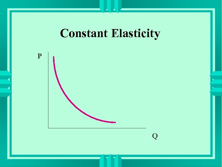Constant Elasticity P Q

Relationship Between Price Elasticity of Demand Total Revenue

Note: Total Revenue (TR) = Total Expenditure. Total revenue is from the firm’s perspective; total expenditure is from the consumer’s perspective. Both are computed by multiplying price by quantity. Thus, TR = P Q

Consider the product of two numbers, Z = XY. Clearly, if both X and Y increase, then the product Z must increase too. Also, if both X and Y decrease, then the product Z must decrease too.

However, if X increases and Y decreases, or vice versa, then whether the product Z increases or decreases depends on the relative magnitude of the changes in X and Y. That is, if X increases a lot and Y decreases a little, then Z will increase. If X increases a little and Y decreases a lot, then Z will decrease. If Y decreases by the same percentage that X increased, then Z will remain unchanged.

The same idea carries over to the concept of total revenue, which is the product of price and quantity: TR = PQ. Generally, when the price of a product increases, the quantity demanded will decrease and vice versa. So, whether TR increases, decreases, or remains the same when the price of a product changes depends on the relative magnitudes of the changes in price and quantity.

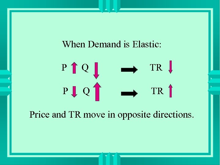When Demand is Elastic: P Q TR Price and TR move in opposite directions.

Example: Elastic Demand When the price of PCs increased from $1600 to $1700, the number of PCs decreased from 500 to 400. The elasticity was -3. 667. Initially, TR = (1600)(500) = 800, 000. Later, TR = (1700)(400) = 680, 000. So TR fell when price increased.

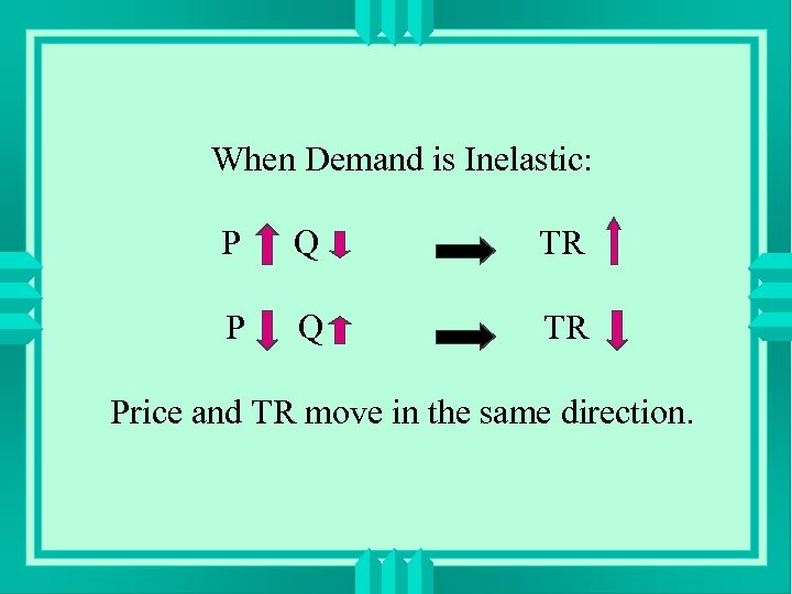When Demand is Inelastic: P Q TR Price and TR move in the same direction.

Example: Inelastic Demand Suppose when the price of a good increased from $90 to $110, the quantity demanded decreased from 210 to 190. The elasticity can be shown to be -0. 5. Initially, TR = (90)(210) = 18, 900. Later, TR = (110)(190) = 20, 900. So TR increased when price increased.

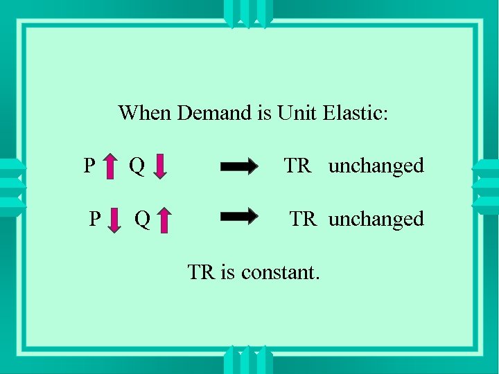When Demand is Unit Elastic: P Q TR unchanged TR is constant.

Example: Unit Elastic Demand Suppose when the price of personal computers increases from $1500 to $1700, the quantity demanded decreases from 850 to 750. Then the elasticity can be shown to be -1. Initially, TR = (1500)(850) = 1, 275, 000. Later, TR = (1700)(750) = 1, 275, 000. So TR is unchanged when price changes.

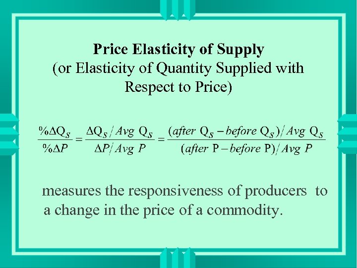Price Elasticity of Supply (or Elasticity of Quantity Supplied with Respect to Price) measures the responsiveness of producers to a change in the price of a commodity.

Example: Suppose the price of personal computers increased from $1550 to $1650. As a result, the number of PCs that area manufacturers were willing to produce per week rose from 490 to 510. Calculate the elasticity of quantity supplied of PCs with respect to the price of PCs.

Calculating as we did for price elasticity of demand, we get price elasticity of supply % qty supplied of PCs % price of PCs = 4 / 6. 25 =. 64 Interpretation: When the price of PCs increases by one percent, the quantity supplied of PCs increases by. 64 percent. Since the elasticity is less than one, quantity supplied of PCs is inelastic with respect to price.

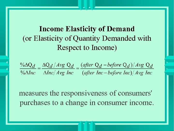Income Elasticity of Demand (or Elasticity of Quantity Demanded with Respect to Income) measures the responsiveness of consumers' purchases to a change in consumer income.

Example: Suppose your income increased from $1000 to $1150 per month. As a result, the number of pounds of potatoes you purchase per month decreased from 10 to 9. Calculate the elasticity of demand for potatoes with respect to income.

Calculating as we have done before, we get income elasticity of demand % qty demanded of potatoes % income = - 10. 53 / 13. 95 = -. 75 Interpretation: When the income increases by one percent, the quantity demanded of potatoes decreases by 0. 75 percent.

Inferior Good a good with a negative income elasticity of demand. The negative sign indicates that income and quantity demanded of the good (potatoes) move in opposite directions. When income rises, people buy less. When income falls, people buy more.

Normal Good a good with a positive income elasticity of demand. For normal goods, when income rises, people buy more. When income falls, people buy less. Most goods are normal goods.

Example: Suppose your income increased from $2000 to $2080 per month. As a result, the number of movies you see per month rose from 4 to 5. Calculate the elasticity of demand for movies with respect to income.

Calculating as before, we get income elasticity of demand for movies % qty demanded of movies % income = 22. 22 / 3. 92 = 5. 668 Interpretation: When the income increases by one percent, the quantity demanded of movies increases by 5. 668 percent. Since the income elasticity of movies is positive, movies are a normal good.

Categorizing goods as normal or inferior Normal good: income elasticity is positive Inferior good: income elasticity is negative Note: Do NOT take the absolute value of the income elasticity when categorizing goods as normal or inferior.

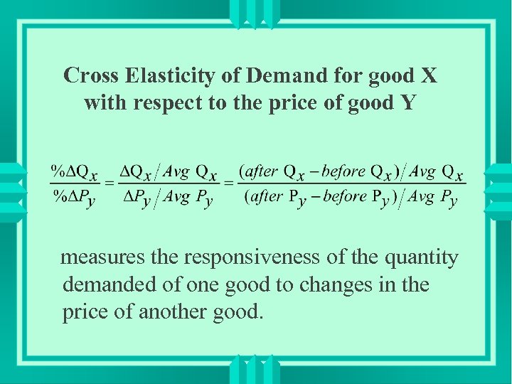Cross Elasticity of Demand for good X with respect to the price of good Y measures the responsiveness of the quantity demanded of one good to changes in the price of another good.

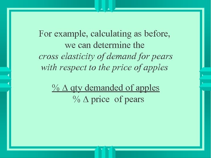For example, calculating as before, we can determine the cross elasticity of demand for pears with respect to the price of apples % qty demanded of apples % price of pears

Substitutes When the cross elasticity between two goods is positive, the two goods are called substitutes. A substitute is a good that can be used instead of another good.

The price of one good and the quantity demanded of the substitute good move in the same direction. When the price of pears decreases, the quantity demanded of apples decreases. When the price of pears increases, the quantity demanded of apples increases.

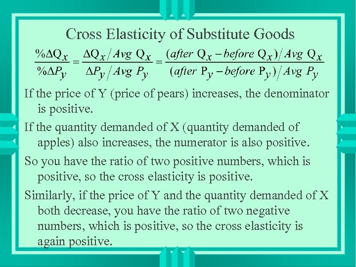Cross Elasticity of Substitute Goods If the price of Y (price of pears) increases, the denominator is positive. If the quantity demanded of X (quantity demanded of apples) also increases, the numerator is also positive. So you have the ratio of two positive numbers, which is positive, so the cross elasticity is positive. Similarly, if the price of Y and the quantity demanded of X both decrease, you have the ratio of two negative numbers, which is positive, so the cross elasticity is again positive.

Complements When the cross elasticity between two goods is negative, the two goods are called complements. A complement is a good that is used along with another good.

The price of one good and the quantity demanded of the complementary good move in opposite directions. When the price of coffee decreases, the quantity demanded of cream increases. When the price of coffee increases, the quantity demanded of cream decreases. So for the cross elasticity of complements, we will have the ratio of a positive number and a negative number. So the cross elasticity will be negative.

Categorizing goods as substitutes or complements Substitutes: cross elasticity is positive Complements: cross elasticity is negative Note: Do NOT take the absolute value of the cross elasticity when categorizing goods as substitutes or complements.

At the website where my lectures are posted, there is also a list that summarizes the formulas for the course. The elasticity formulas are on that list.

The Effect of Elasticity on the Burden of a Tax

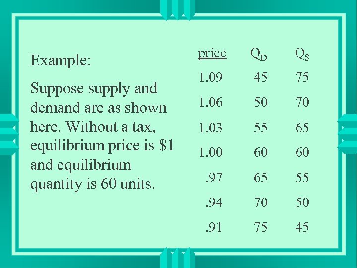Example: Suppose supply and demand are as shown here. Without a tax, equilibrium price is $1 and equilibrium quantity is 60 units. price QD QS 1. 09 45 75 1. 06 50 70 1. 03 55 65 1. 00 60 60 . 97 65 55 . 94 70 50 . 91 75 45

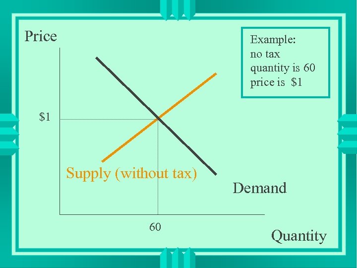Price Example: no tax quantity is 60 price is $1 $1 Supply (without tax) 60 Demand Quantity

Now suppose a tax of six cents per unit is imposed. Then, from the buyer’s view, for each quantity supplied, the total price per unit is six cents higher than before. (Equivalently, for a given total price per unit, suppliers are willing to provide fewer units than before. ) So the buyers see a new supply curve.

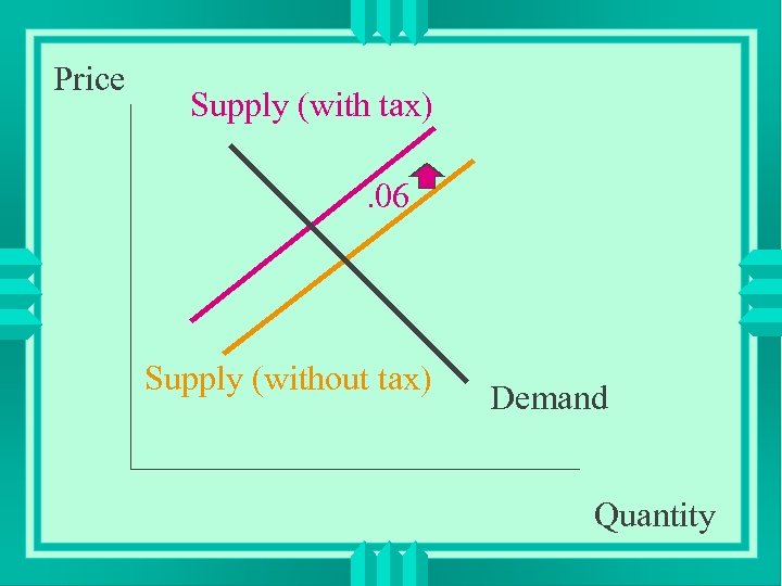Price Supply (with tax). 06 Supply (without tax) Demand Quantity

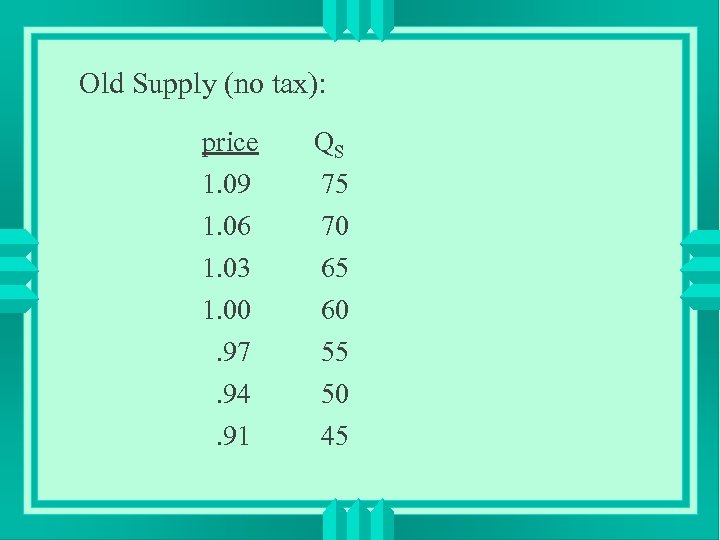Old Supply (no tax): price QS 1. 09 75 1. 06 70 1. 03 1. 00. 97. 94. 91 65 60 55 50 45

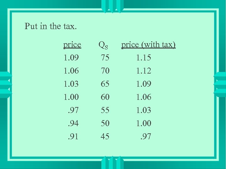Put in the tax. price QS price (with tax) 1. 09 75 1. 15 1. 06 70 1. 12 1. 03 1. 00. 97. 94. 91 65 60 55 50 45 1. 09 1. 06 1. 03 1. 00. 97

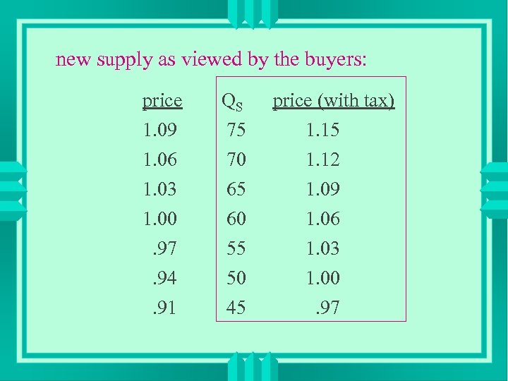new supply as viewed by the buyers: price QS price (with tax) 1. 09 75 1. 15 1. 06 70 1. 12 1. 03 1. 00. 97. 94. 91 65 60 55 50 45 1. 09 1. 06 1. 03 1. 00. 97

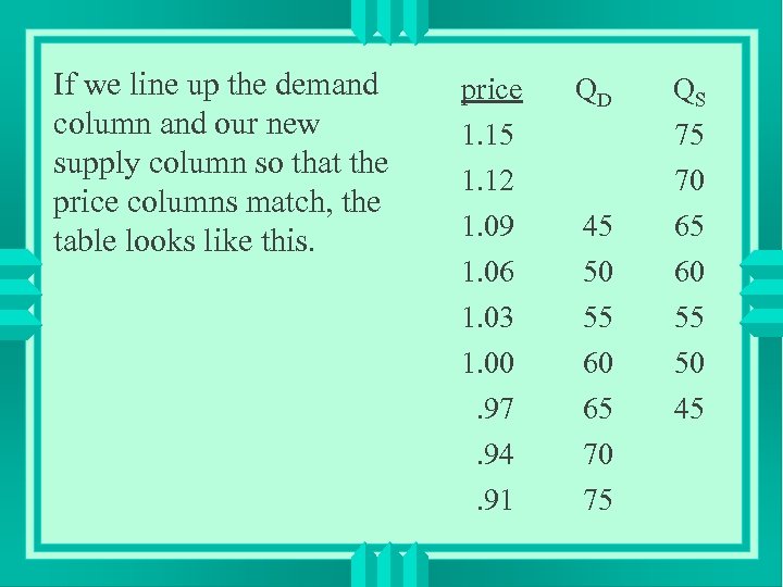If we line up the demand column and our new supply column so that the price columns match, the table looks like this. price QD QS 1. 15 75 1. 12 70 1. 09 1. 06 1. 03 1. 00. 97. 94. 91 45 50 55 60 65 70 75 65 60 55 50 45

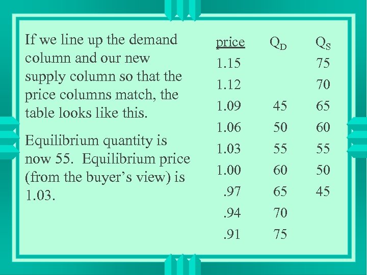If we line up the demand column and our new supply column so that the price columns match, the table looks like this. Equilibrium quantity is now 55. Equilibrium price (from the buyer’s view) is 1. 03. price QD QS 1. 15 75 1. 12 70 1. 09 1. 06 1. 03 1. 00. 97. 94. 91 45 50 55 60 65 70 75 65 60 55 50 45

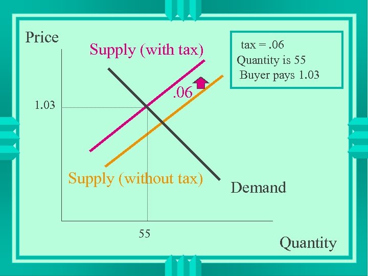Price Supply (with tax) tax =. 06 Quantity is 55 Buyer pays 1. 03 . 06 1. 03 Supply (without tax) 55 Demand Quantity

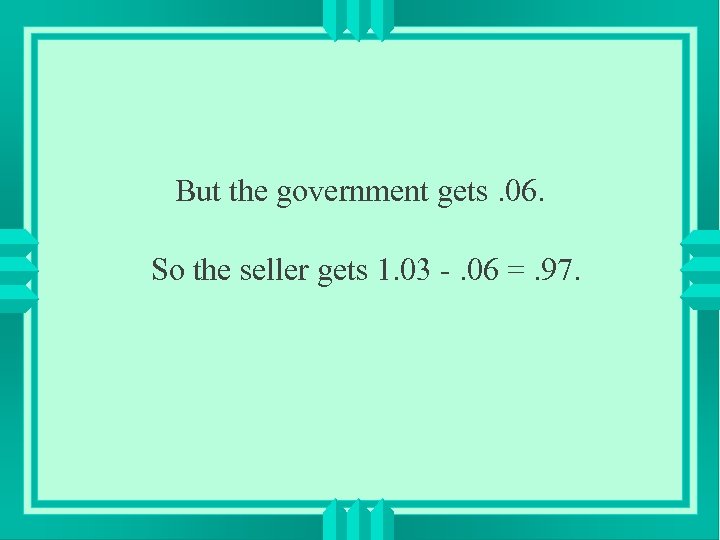But the government gets. 06. So the seller gets 1. 03 -. 06 =. 97.

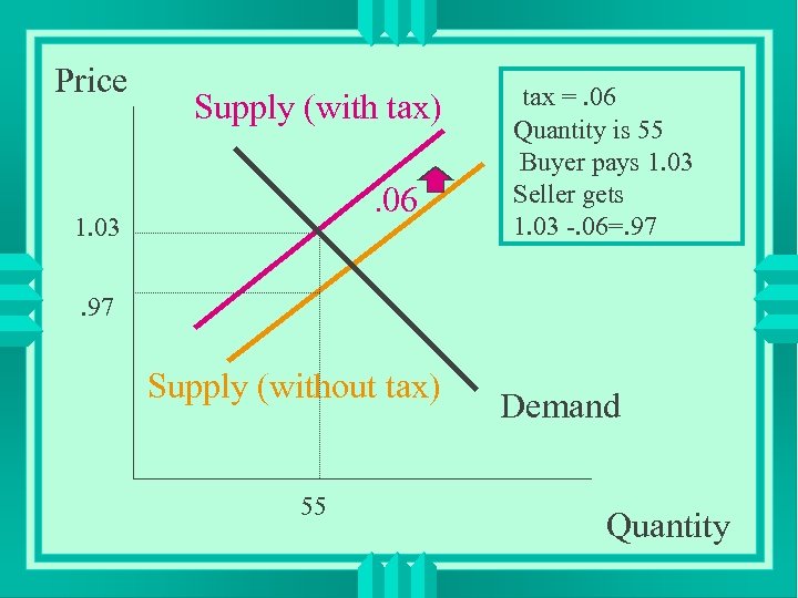Price Supply (with tax). 06 1. 03 tax =. 06 Quantity is 55 Buyer pays 1. 03 Seller gets 1. 03 -. 06=. 97 Supply (without tax) 55 Demand Quantity

The burden of the tax is shared evenly in this example. The buyer pays three cents more per unit than before the tax and the seller gets three cents less per unit.

With the tax, the buyer pays more and the seller receives less than without the tax. The burden of the tax is shared.

Suppose the elasticity of demand is smaller. The demand curve is steeper. How does this affect how the tax burden is divided?

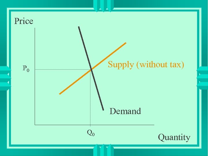Price Supply (without tax) P 0 Demand Q 0 Quantity

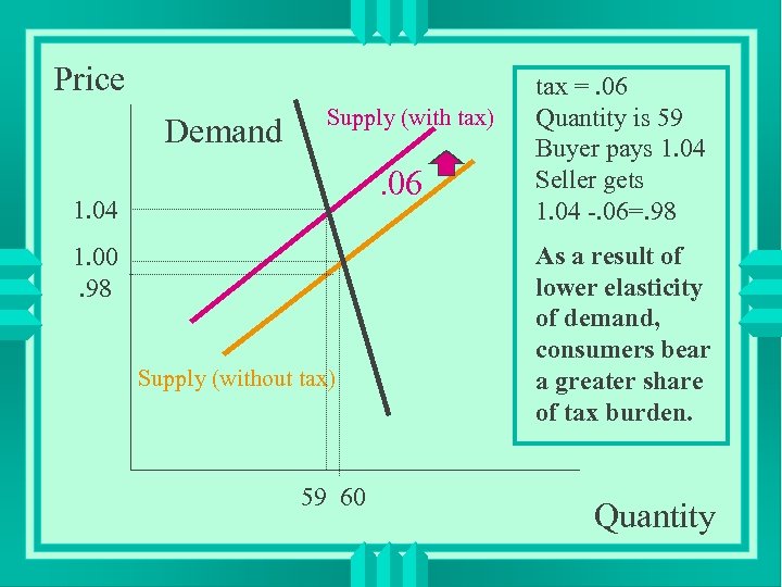Price Demand Supply (with tax) . 06 1. 04 1. 00. 98 Supply (without tax) 59 60 tax =. 06 Quantity is 59 Buyer pays 1. 04 Seller gets 1. 04 -. 06=. 98 As a result of lower elasticity of demand, consumers bear a greater share of tax burden. Quantity

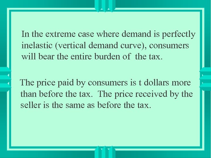In the extreme case where demand is perfectly inelastic (vertical demand curve), consumers will bear the entire burden of the tax. The price paid by consumers is t dollars more than before the tax. The price received by the seller is the same as before the tax.

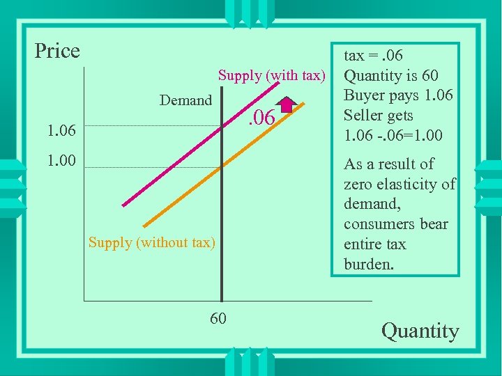Price Supply (with tax) Demand 1. 06 1. 00 Supply (without tax) 60 . 06 tax =. 06 Quantity is 60 Buyer pays 1. 06 Seller gets 1. 06 -. 06=1. 00 As a result of zero elasticity of demand, consumers bear entire tax burden. Quantity

When supply is less elastic and sellers are less responsive to price changes, sellers will bear a larger share of the tax burden, and buyers will bear a smaller share.

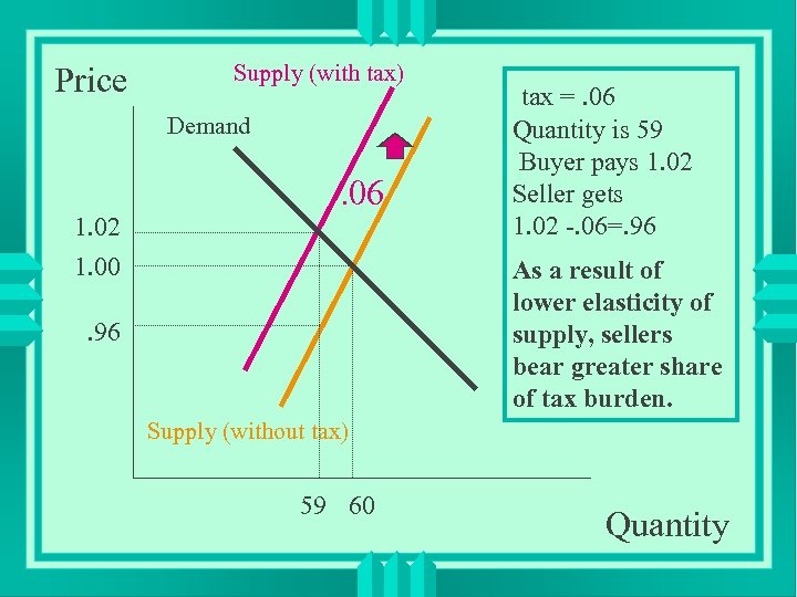Price Supply (with tax) Demand 1. 02 . 06 1. 00 tax =. 06 Quantity is 59 Buyer pays 1. 02 Seller gets 1. 02 -. 06=. 96 As a result of lower elasticity of supply, sellers bear greater share of tax burden. . 96 Supply (without tax) 59 60 Quantity

In the extreme case where supply is perfectly inelastic (vertical supply curve), sellers will bear the entire burden of the tax. The price received by sellers is t dollars less than before the tax. The price paid by consumers is the same as before the tax.

Elasticity & Tax Burden Conclusions When demand is less elastic and consumers are less responsive to price changes, consumers bear a larger share of the tax burden, and sellers bear a smaller share. When supply is less elastic and firms are less responsive to price changes, firms bear a larger share of the tax burden, and consumers bear a smaller share.