Elasticity of Demand Supply Chap 18 —

Elasticity of Demand & Supply Chap 18 - Extensions of Demand & Supply Analysis – Mc. Connel & Brue Chap 2 -The Basics of Demand & Supply – Pindyck Lecture 7

Price Elasticity of Supply: The Market Period • The market period is the period that occurs when the time immediately after a change in market price is too short for producers to respond with a change in quantity supplied. • E. g. the supply for tomatoes is perfectly inelastic (vertical); the farmer will sell the truckload whether the price is high or low. • The farmer does not have time to respond to a change in demand from D 1 to D 2 (p 349 -Ch 18)

Price Elasticity of Supply: The Short Run • The short run is a period of time too short to change plant capacity but long enough to use fixed plant more or less intensively • The farmer does have time in the short run to cultivate tomatoes more intensively by employing more labor, more fertilizer and pesticides to the crop- even though his land machinery is fixed • The result is greater output in response to an increase in demand, as supply of tomatoes is more elastic.

Price Elasticity of Supply: The Long Run • The long run is a time period long enough for farmers to adjust their plant sizes for new firms to enter (or exit) the industry • The farmer has time to acquire additional land buy more machinery and equipment • Other farmers may switch to tomato farming in response to the increased demand – Therefore supply curve is more elastic than short run

Supply & Total Revenue • There is no total revenue test for elasticity of supply • Supply shows a positive or direct relationship between price and amount supplied • Regardless of the degree of elasticity or inelasticity, price and total revenue always move together.

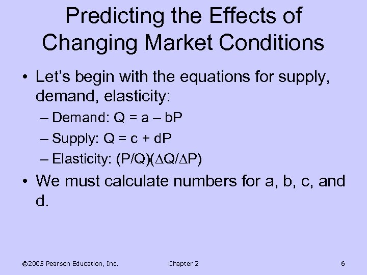Predicting the Effects of Changing Market Conditions • Let’s begin with the equations for supply, demand, elasticity: – Demand: Q = a – b. P – Supply: Q = c + d. P – Elasticity: (P/Q)( Q/ P) • We must calculate numbers for a, b, c, and d. © 2005 Pearson Education, Inc. Chapter 2 6

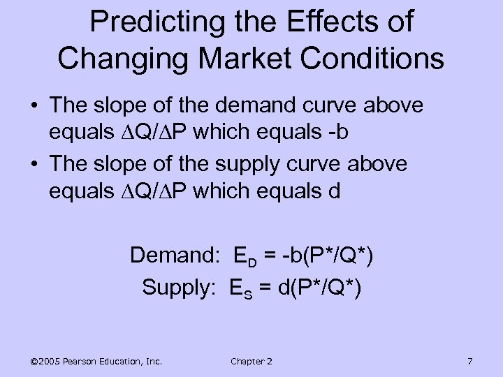Predicting the Effects of Changing Market Conditions • The slope of the demand curve above equals Q/ P which equals -b • The slope of the supply curve above equals Q/ P which equals d Demand: ED = -b(P*/Q*) Supply: ES = d(P*/Q*) © 2005 Pearson Education, Inc. Chapter 2 7

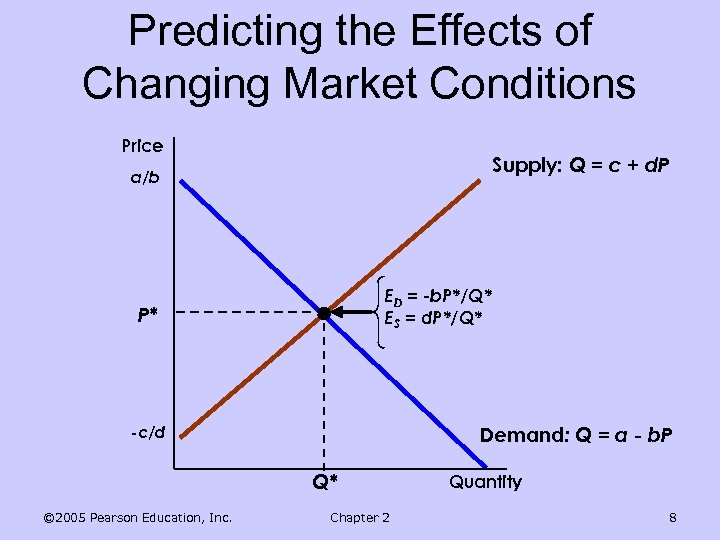Predicting the Effects of Changing Market Conditions Price Supply: Q = c + d. P a/b ED = -b. P*/Q* ES = d. P*/Q* P* Demand: Q = a - b. P -c/d Q* © 2005 Pearson Education, Inc. Chapter 2 Quantity 8

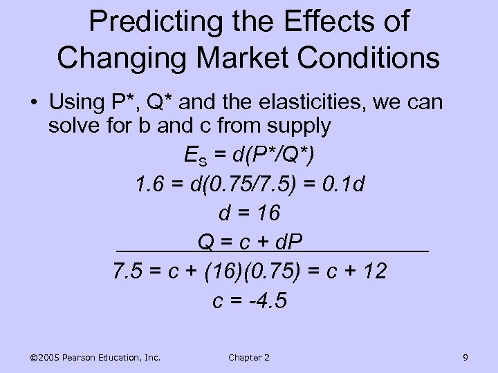Predicting the Effects of Changing Market Conditions • Using P*, Q* and the elasticities, we can solve for b and c from supply ES = d(P*/Q*) 1. 6 = d(0. 75/7. 5) = 0. 1 d d = 16 Q = c + d. P 7. 5 = c + (16)(0. 75) = c + 12 c = -4. 5 © 2005 Pearson Education, Inc. Chapter 2 9

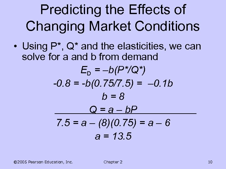Predicting the Effects of Changing Market Conditions • Using P*, Q* and the elasticities, we can solve for a and b from demand ED = –b(P*/Q*) -0. 8 = -b(0. 75/7. 5) = – 0. 1 b b=8 Q = a – b. P 7. 5 = a – (8)(0. 75) = a – 6 a = 13. 5 © 2005 Pearson Education, Inc. Chapter 2 10

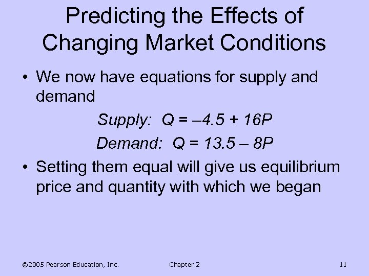Predicting the Effects of Changing Market Conditions • We now have equations for supply and demand Supply: Q = – 4. 5 + 16 P Demand: Q = 13. 5 – 8 P • Setting them equal will give us equilibrium price and quantity with which we began © 2005 Pearson Education, Inc. Chapter 2 11

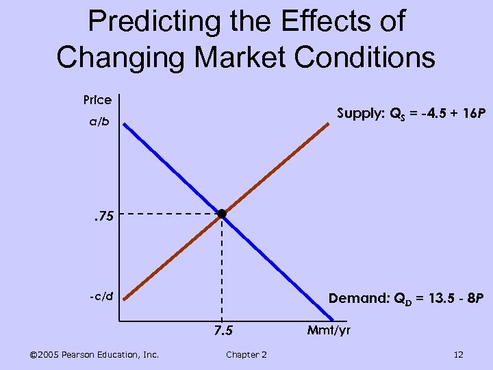Predicting the Effects of Changing Market Conditions Price Supply: QS = -4. 5 + 16 P a/b . 75 Demand: QD = 13. 5 - 8 P -c/d 7. 5 © 2005 Pearson Education, Inc. Chapter 2 Mmt/yr 12

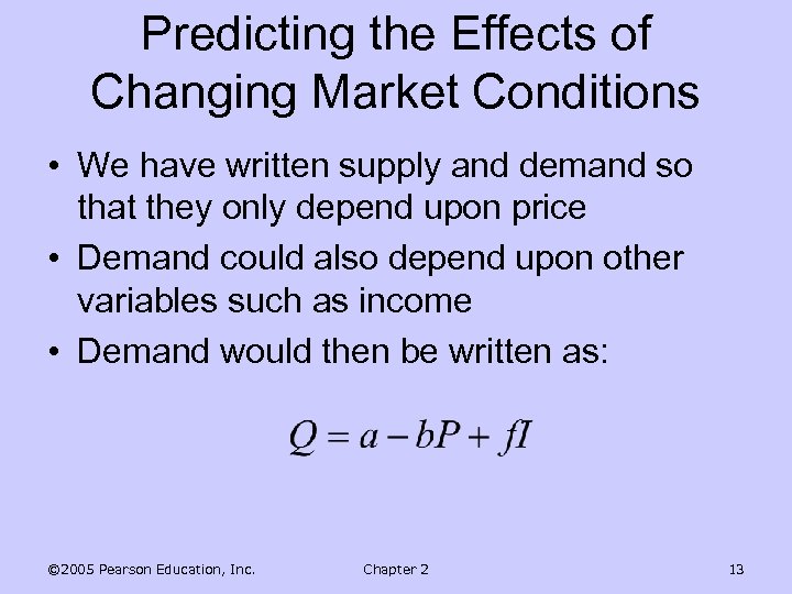Predicting the Effects of Changing Market Conditions • We have written supply and demand so that they only depend upon price • Demand could also depend upon other variables such as income • Demand would then be written as: © 2005 Pearson Education, Inc. Chapter 2 13

Consumer & Producer Surplus • The difference between the maximum price a consumer is willing to pay for a product and the actual price (p 352 -Ch 18) • Producer Surplus is the difference between the actual price a producer receives and the minimum acceptable price

• Productive efficiency is achieved because competition forces producers to use the best techniques and combinations of resources in producing goods • Allocative efficiency is achieved because the correct quantity of output is produced relative to other goods and services • Demand Curve measures marginal benefit of oranges at each level of output • Supply Curve measures marginal cost

Allocative Efficiency • Allocative Efficiency : – MC = MB – Maximum willingness to pay = minimum acceptable price – Combined consumer and producer is at its maximum • Where maximum willingness to pay for the last unit equals minimum acceptable price for that unit, does the society exhaust all the opportunities to add to combined consumer and producer surplus

Short-Run Versus Long-Run Elasticity • Most goods and services: – Long-run price elasticity of supply is greater than short-run price elasticity of supply • Other Goods (durables, recyclables): – Long-run price elasticity of supply is less than short-run price elasticity of supply © 2005 Pearson Education, Inc. Chapter 2 17

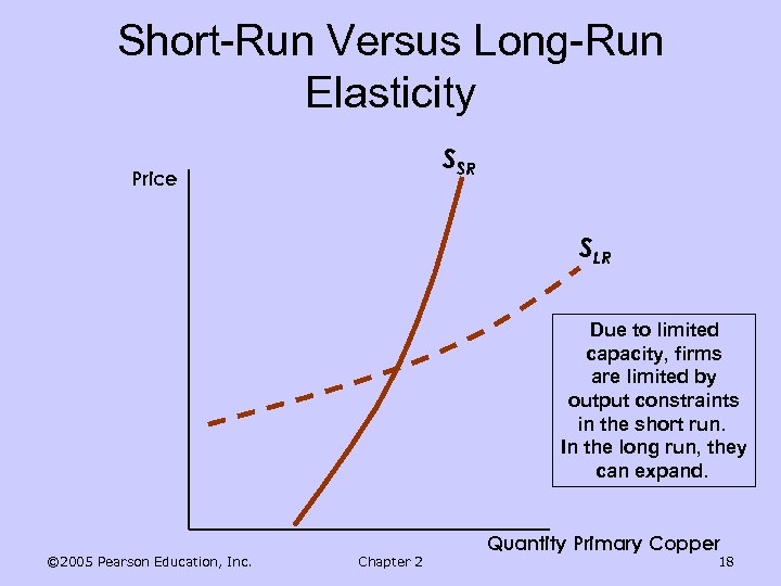Short-Run Versus Long-Run Elasticity SSR Price SLR Due to limited capacity, firms are limited by output constraints in the short run. In the long run, they can expand. © 2005 Pearson Education, Inc. Chapter 2 Quantity Primary Copper 18

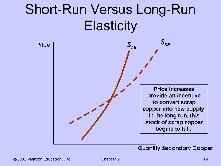Short-Run Versus Long-Run Elasticity SLR Price SSR Price increases provide an incentive to convert scrap copper into new supply. In the long run, this stock of scrap copper begins to fall. Quantity Secondary Copper © 2005 Pearson Education, Inc. Chapter 2 19

Short-Run Versus Long-Run Elasticity • Price elasticity varies with the amount of time consumers have to respond to a price • Short-run demand supply curves often look very different from their long-run counterparts © 2005 Pearson Education, Inc. Chapter 2 20

Short-Run Versus Long-Run Elasticity • Demand – In general, demand is much more price elastic in the long run • Consumers take time to adjust consumption habits • Demand might be linked to another good that changes slowly • More substitutes are usually available in the long run © 2005 Pearson Education, Inc. Chapter 2 21

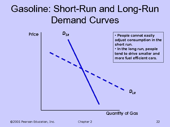Gasoline: Short-Run and Long-Run Demand Curves Price DSR • People cannot easily adjust consumption in the short run. • In the long run, people tend to drive smaller and more fuel efficient cars. DLR Quantity of Gas © 2005 Pearson Education, Inc. Chapter 2 22

Short-Run Versus Long-Run Elasticity • Demand Durability – For some durable goods, demand is more elastic in the short run – If goods are durable, then when price increases, consumers choose to hold on to the good instead of replacing it – But in long run, older durable goods will have to be replaced © 2005 Pearson Education, Inc. Chapter 2 23

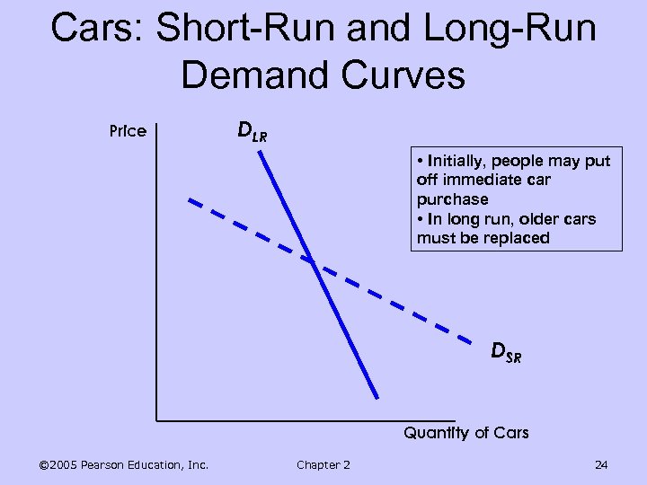Cars: Short-Run and Long-Run Demand Curves Price DLR • Initially, people may put off immediate car purchase • In long run, older cars must be replaced DSR Quantity of Cars © 2005 Pearson Education, Inc. Chapter 2 24

Short-Run Versus Long-Run Elasticity • Income elasticity also varies with the amount of time consumers have to respond to an income change – For most goods and services, income elasticity is higher in the long run – When income changes, it takes time to adjust spending © 2005 Pearson Education, Inc. Chapter 2 25

Short-Run Versus Long-Run Elasticity • Income elasticity of durable goods – Income elasticity is smaller in the long run than in the short run • Increases in income mean consumers will want to hold more cars • Once older cars are replaced, purchases will only be to replace old cars • Less purchases from income increase in long run than in short run © 2005 Pearson Education, Inc. Chapter 2 26