Efficient Process-Hotspot Detection Using Range Pattern Matching in

Efficient Process-Hotspot Detection Using Range Pattern Matching in Routing Stage Hailong Yao 1 Subarna Sinha 2 Charles Chiang 2 Xianlong Hong 1 Yici Cai 1 1 Department of Computer Science and Technology Tsinghua University, Beijing, P. R. China 2 Synopsys ATG, Mountain View, CA This work is done during the author’s internship at Synopsys ATG

Outline l Motivation l Range Patterns and Matching l Process-Hotspot Detection System l Experimental Results l Conclusion

Motivation l Manufacturability-aware physical design is becoming a necessity l Certain layout configurations susceptible to stress and lithographic process fluctuations affect yield l Process-hotspots: layout configurations most susceptible to process issues l Remove process-hotspots and replace them with more yield-friendly configurations

Limitations of Recommended Rules l Fabs use design rules (like recommended rules) to represent process-hotspots l Limitations: Some effects are non-local ¤ Difficult to represent relationships between large group of non-neighboring objects with a small set of rules ¤ Explosion of design rules slows down the router ¤ DRC tools are being supplemented with accurate process simulators (for instance, for lithography) ¤

Limitations of Process Models l Lida Huang, et al at DAC’ 04 [1] and J. Mitra, et al at DAC’ 05 [2] proposed embedding an aerial image simulator in the router to identify process-hotspots l Limitations: Lack of knowledge of downstream steps and overestimation of process-hotspots ¤ Huge computational expense ¤ [1] L. -D. Huang and M. D. F. Wong, “Optical proximity correction (OPC)friendly maze routing, ” In DAC, pages 186– 191, June 2004. [2] J. Mitra, P. Yu, and D. Z. Pan, “RADAR: Ret-aware detailed routing using fast lithography simulations, ” In DAC, pages 369– 372, June 2005.

Represent Process-hotspots with Patterns l A good representation of process-hotspots would be a 2 D layout of rectangles, i. e. a pattern l Can be built off-line using test-structures or more accurate simulation tools l Process-hotspot detection during routing would complement current advances in yield enabling steps

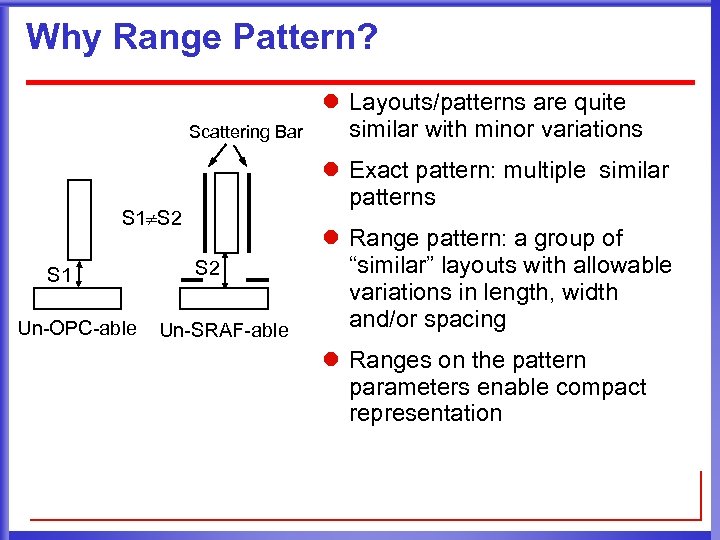Why Range Pattern? Scattering Bar l Exact pattern: multiple similar patterns S 1 S 2 S 1 Un-OPC-able l Layouts/patterns are quite similar with minor variations S 2 Un-SRAF-able l Range pattern: a group of “similar” layouts with allowable variations in length, width and/or spacing l Ranges on the pattern parameters enable compact representation

Process-hotspot Detection l Collaborate with a fab or in-house accurate simulation and mask synthesis flows to build range patterns l Score the patterns in the set based on yield impact l Scores can be used by the router to give higher priority during correction l Represent process-hotspots as a library of range patterns l Process-hotspot detection: find all the locations where the layout is identical to one of the patterns contained in a range pattern

Outline l Motivation l Range Patterns and Matching ¤ ¤ ¤ Range Pattern Definitions Layout Representation Range Pattern Representation l Process-Hotspot Detection System l Experimental Results l Conclusion

Range Pattern Definitions l Range pattern: DRC-correct two-dimensional layout of rectangles with additional specifications: 1. 2. 3. 4. Widths and lengths of the rectangles can vary within certain user-specified bounds Spacings between pairs of rectangles can vary within certain user-specified bounds Optimal widths and lengths of the rectangles and optimal spacings between pairs of rectangles can be specified Constraints can be specified over linear combinations of the widths, lengths and spacings of the rectangles

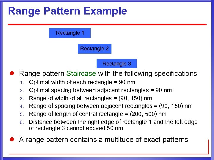Range Pattern Example Rectangle 1 Rectangle 2 Rectangle 3 l Range pattern Staircase with the following specifications: 1. 2. 3. 4. 5. 6. Optimal width of each rectangle = 90 nm Optimal spacing between adjacent rectangles = 90 nm Range of width of all rectangles = (90, 150) nm Range of spacing between adjacent rectangles = (90, 150) nm Range of length of central rectangle = (200, 500) nm Distance between the right edge of rectangle 1 and the left edge of rectangle 3 cannot exceed 50 nm l A range pattern contains a multitude of exact patterns

Range Pattern Matching Problem l The Range Pattern Matching (RPM) problem: Given a layout and a range pattern, determine all occurrences of the range pattern in the layout and score these occurrences using the scoring mechanism for the range pattern

Outline l Motivation l Range Patterns and Matching ¤ ¤ ¤ Range Pattern Definitions Layout Representation Range Pattern Representation l Process-Hotspot Detection System l Experimental Results l Conclusion

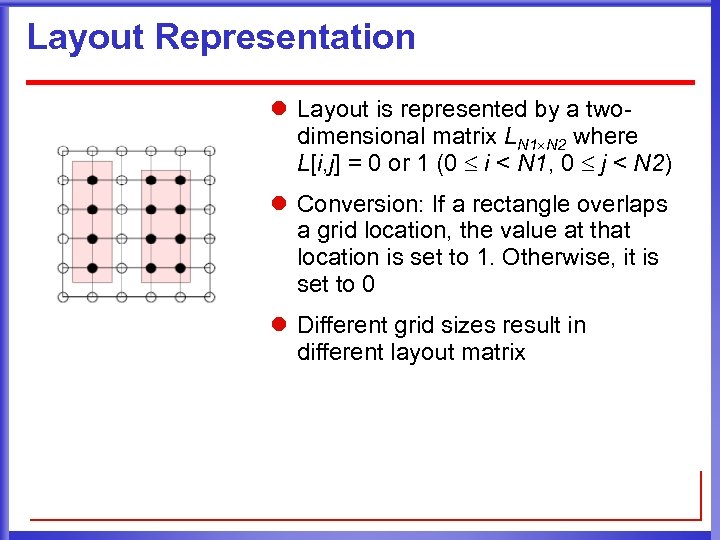Layout Representation l Layout is represented by a twodimensional matrix LN 1 N 2 where L[i, j] = 0 or 1 (0 i < N 1, 0 j < N 2) l Conversion: If a rectangle overlaps a grid location, the value at that location is set to 1. Otherwise, it is set to 0 l Different grid sizes result in different layout matrix

Outline l Motivation l Range Patterns and Matching ¤ ¤ ¤ Range Pattern Definitions Layout Representation Range Pattern Representation l Process-Hotspot Detection System l Experimental Results l Conclusion

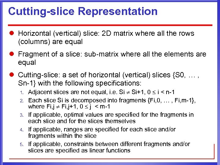Cutting-slice Representation l Horizontal (vertical) slice: 2 D matrix where all the rows (columns) are equal l Fragment of a slice: sub-matrix where all the elements are equal l Cutting-slice: a set of horizontal (vertical) slices {S 0, … , Sn-1} with the following specifications: 1. 2. 3. 4. 5. Adjacent slices are not equal, i. e. Si Si+1, 0 i < n-1 Each slice Si is decomposed into fragments {Fi, 0, … , Fi, m-1}, where Fi, j+1, 0 j < m-1 If applicable, optimal values are specified for the fragments in each slice and for the slices themselves If applicable, ranges are specified for each slice and/or fragments within the slice If applicable, constraints between different fragments and/or slices are specified as linear functions

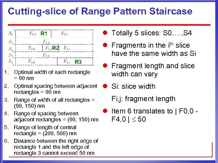Cutting-slice of Range Pattern Staircase l Totally 5 slices: S 0, …, S 4 R 1 l Fragments in the ith slice have the same width as Si R 2 R 3 1. Optimal width of each rectangle = 90 nm 2. Optimal spacing between adjacent rectangles = 90 nm 3. Range of width of all rectangles = (90, 150) nm 4. Range of spacing between adjacent rectangles = (90, 150) nm 5. Range of length of central rectangle = (200, 500) nm 6. Distance between the right edge of rectangle 1 and the left edge of rectangle 3 cannot exceed 50 nm l Fragment length and slice width can vary l Si: slice width Fi, j: fragment length l Item 6 translates to | F 0, 0 F 4, 0 | 50

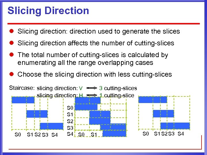Slicing Direction l Slicing direction: direction used to generate the slices l Slicing direction affects the number of cutting-slices l The total number of cutting-slices is calculated by enumerating all the range overlapping cases l Choose the slicing direction with less cutting-slices Staircase: slicing direction: V slicing direction: H S 0 S 1 S 2 S 3 S 4 S 0 3 cutting-slices 1 cutting-slice S 1 S 2 S 3 S 0 S 1 S 2 S 3 S 4

Outline l Motivation l Range Patterns and Matching l Process-Hotspot Detection System ¤ ¤ ¤ Overview Range Pattern Matching Sub-problem Scalability and Runtime Optimization l Experimental Results l Conclusion

Overview l Hierarchical dual-grid scheme with matching done on two grid sizes l The grid sizes are used to generate the layout matrices and the cutting-slices of the range pattern l Matching with the coarse grid identifies locations that are potential matches l Match locations are verified on the finer grid size l Fine grid size is equal to the manufacturing grid size

Outline l Motivation l Range Patterns and Matching l Process-Hotspot Detection System ¤ ¤ ¤ Overview Range Pattern Matching Sub-problem Scalability and Runtime Optimization l Experimental Results l Conclusion

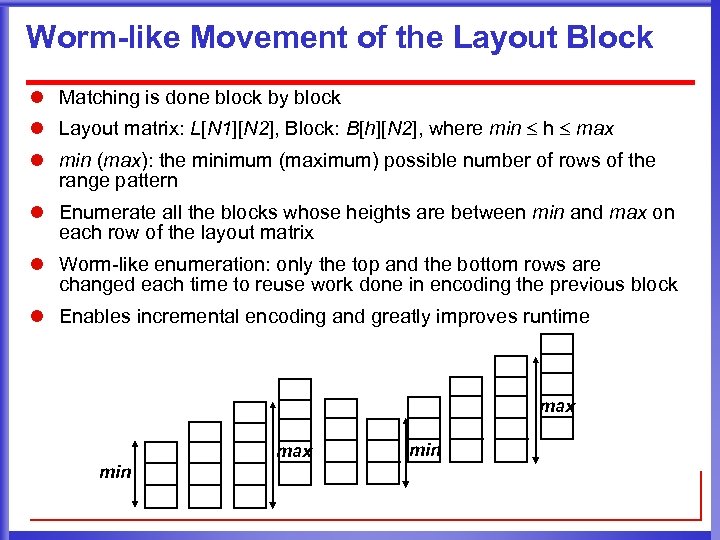Worm-like Movement of the Layout Block l Matching is done block by block l Layout matrix: L[N 1][N 2], Block: B[h][N 2], where min h max l min (max): the minimum (maximum) possible number of rows of the range pattern l Enumerate all the blocks whose heights are between min and max on each row of the layout matrix l Worm-like enumeration: only the top and the bottom rows are changed each time to reuse work done in encoding the previous block l Enables incremental encoding and greatly improves runtime max min

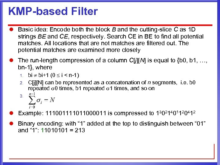KMP-based Filter l Basic idea: Encode both the block B and the cutting-slice C as 1 D strings BE and CE, respectively. Search CE in BE to find all potential matches. All locations that are not matches are filtered out. The potential matches are examined more closely l The run-length compression of a column C[j][N] is equal to {b 0, b 1, …, bn-1}, where 1. 2. bi+1 (0 i < n-1) C[j][N] can be represented as a concatenation of n segments, i. e. b 0 repeated 0 times, b 1 repeated 1 times, and so on 3. l Example: 111001111011000011 is compressed to 13021401120412 l Binary encoding: with “ 1” added at the top to distinguish between “ 01” and “ 1”: 11010101 = 213

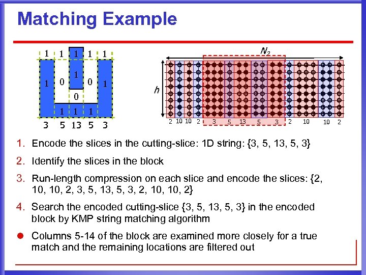Matching Example 1 1 1 0 1 0 3 N 2 1 1 1 h 1 1 1 5 13 5 3 2 10 10 2 3 5 13 5 3 2 10 1. Encode the slices in the cutting-slice: 1 D string: {3, 5, 13, 5, 3} 2. Identify the slices in the block 3. Run-length compression on each slice and encode the slices: {2, 10, 2, 3, 5, 13, 5, 3, 2, 10, 2} 4. Search the encoded cutting-slice {3, 5, 13, 5, 3} in the encoded block by KMP string matching algorithm l Columns 5 -14 of the block are examined more closely for a true match and the remaining locations are filtered out 10 2

Complexity Analysis of the RPM Algorithm l Layout matrix: L[N 1][N 2] , Layout block: B[h][N 2] where min h max l Slice identification: O(N 2) l Let the number of identified slices be s (1 s N 2), run-length compression takes O(s U), where U is the average time for updating the run-length compression of each slice l Incremental binary encoding: O(s) l KMP string matching: O(s) l The verification process for each potential match: O(1) l RPM algorithm for one layout block: max(N 2, s U) l Total number of different blocks in the layout matrix L[N 1][N 2] is less than (N 1 -min+1) (max-min+1) l Total time complexity: O(max(N 2, s U) (N 1 -min+1) (max-min+1)) l Key factors: Size of the layout (N 1, N 2), the variation range in the height of the cutting-slice (min, max)

Outline l Motivation l Range Patterns and Matching l Process-Hotspot Detection System ¤ ¤ ¤ Overview Range Pattern Matching Sub-problem Scalability and Runtime Optimization l Experimental Results l Conclusion

Scalability and Runtime Optimization l Scalability: window-by-window matching l Consecutive windows overlap to avoid loss of matches l Runtime: matching on a fine grid size is slow l Hierarchical matching strategy: dual grid matching scheme of coarse grid matching followed by fine grid matching

Outline l Motivation l Range Patterns and Matching l Process-Hotspot Detection System l Experimental Results l Conclusion

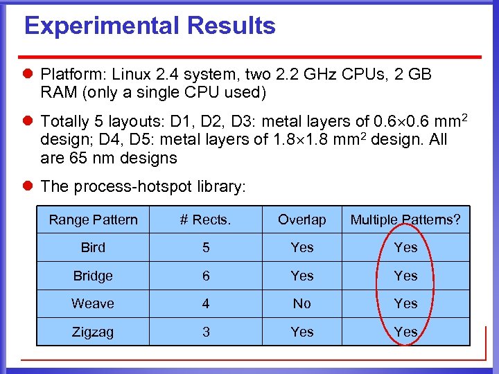Experimental Results l Platform: Linux 2. 4 system, two 2. 2 GHz CPUs, 2 GB RAM (only a single CPU used) l Totally 5 layouts: D 1, D 2, D 3: metal layers of 0. 6 mm 2 design; D 4, D 5: metal layers of 1. 8 mm 2 design. All are 65 nm designs l The process-hotspot library: Range Pattern # Rects. Overlap Multiple Patterns? Bird 5 Yes Bridge 6 Yes Weave 4 No Yes Zigzag 3 Yes

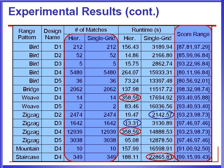Experimental Results (cont. ) Range Pattern Design Name # of Matches Hier. Runtime (s) Single-Grid Hier. 212 156. 43 Single-Grid Score Range Bird D 1 212 Bird D 2 52 52 14. 86 2166. 80 [85. 99, 96. 84] Bird D 3 5 5 15. 75 2862. 74 [93. 22, 96. 84] Bird D 4 5480 264. 07 15933. 31 [80. 11, 96. 84] Bird D 5 36 Bridge D 1 Weave 36 3189. 94 [87. 81, 97. 29] 73. 24 13397. 48 [80. 56, 92. 01] 2062 137. 98 11517. 72 [98. 32, 98. 74] D 4 14 14 358. 59 17694. 92 [93. 40, 95. 88] Weave D 5 2 2 83. 46 16036. 56 [93. 40, 93. 40] Zigzag D 2 2474 19. 47 2142. 57 [93. 23, 98. 73] Zigzag D 3 1642 13. 31 3130. 89 [97. 46, 97. 46] Zigzag D 4 12939 358. 59 14888. 53 [93. 23, 98. 73] Zigzag D 5 3038 Mountain D 4 Staircase D 4 3038 95. 08 12878. 50 [97. 46, 97. 46] 10 10 157. 99 16598. 91 [91. 00, 92. 50] 349 188. 11 22865. 83 [99. 15, 99. 43]

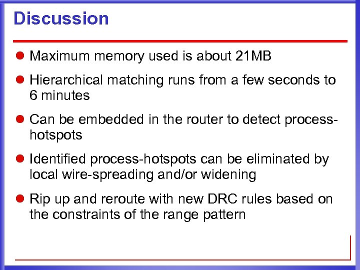Discussion l Maximum memory used is about 21 MB l Hierarchical matching runs from a few seconds to 6 minutes l Can be embedded in the router to detect processhotspots l Identified process-hotspots can be eliminated by local wire-spreading and/or widening l Rip up and reroute with new DRC rules based on the constraints of the range pattern

Outline l Motivation l Range Patterns and Matching l Process-Hotspot Detection System l Experimental Results l Conclusion

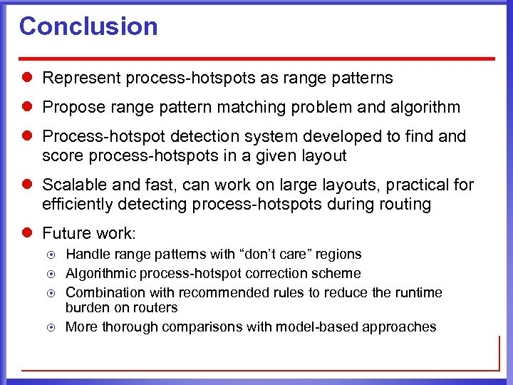Conclusion l Represent process-hotspots as range patterns l Propose range pattern matching problem and algorithm l Process-hotspot detection system developed to find and score process-hotspots in a given layout l Scalable and fast, can work on large layouts, practical for efficiently detecting process-hotspots during routing l Future work: ¤ ¤ Handle range patterns with “don’t care” regions Algorithmic process-hotspot correction scheme Combination with recommended rules to reduce the runtime burden on routers More thorough comparisons with model-based approaches