

5d728aef9882aa1228f56ffe0c9c8ed2.ppt
- Количество слайдов: 69
 Effetto “setaccio” in un gel uniforme
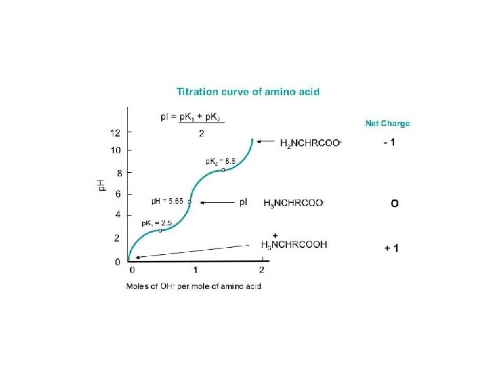
 ELETTROFORESI Migrazione di particelle cariche sotto l’azione di un campo elettrico. Tecnica soprattutto ANALITICA ma anche PREPARATIVA. E’ un mezzo di separazione molto potente, fra i piu’ usati in biochimica Forza elettrica : Fel = q · E Forza frizionale : Ffr = f ·v (f = 6 r ) Quando le forze si bilanciano: q ·E = f ·v q v= —·E f mobilita’ elettroforetica : v q = — E f
 Formazione di un gel di poliacrilammide
 NBT Nitro Blu di Tetrazolio Coomassie Blu
 Locus A 3 alleles Locus B a allele
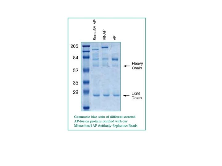
") Western blotting (blotting di proteine)
Western blotting (blotting di proteine)
 • 284 T. officinale samples from a 500 m× 500") Solbrig and Simpson (1974) • 284 T. officinale samples from a 500 m× 500 m area in Ann Arbor, Michigan. • Electrophoretic variations (allozymes) of six enzymes were analyzed
Solbrig and Simpson (1974) • 284 T. officinale samples from a 500 m× 500 m area in Ann Arbor, Michigan. • Electrophoretic variations (allozymes) of six enzymes were analyzed
 Most Commonly Used Molecular Markers in Plants • • RFLP RAPD AFLP SSR & STS
 DNA extraction • From any tissue but: • - Young leaves still actively dividing, so more DNA available. • - Older plant parts beginning to senesce, and DNA is breaking down so less useful. • From any condition plant, but green-house or growthchamber materials tend to be cleaner (less fungus, dirt carrying bacteria, insects, etc).
 • Extracted") DNA extraction • Extracted DNA checked for quantity (spectrophotometer or quality gel) • Extracted DNA checked for quality (quality gel)
DNA extraction • Extracted DNA checked for quantity (spectrophotometer or quality gel) • Extracted DNA checked for quality (quality gel)
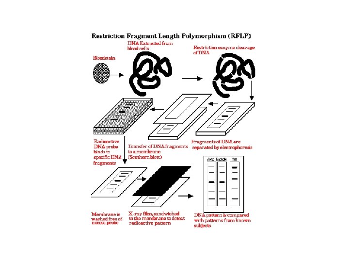
 RFLP: Restriction Fragment Length Polymorphism • Plant genomic DNA digested with restriction endonuclease • DNA fragments separated via electrophoresis and transferred to non-charged membranes • Membranes exposed to probes labeled with digoxigenin or P 32 via southern hybridization • Film exposed to the x-ray or light labeled membranes
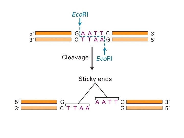
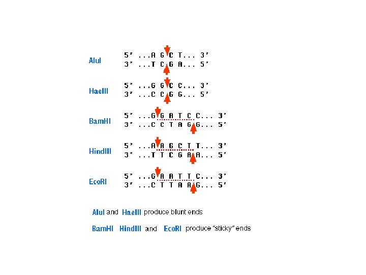
 other methods of detecting DNA sequence variations * RFLP: restriction fragment length polymorphism restriction endonucleases: enzymes that cleave DNA at specific places the produced DNA fragments are separated by electrophoresis restriction sites are gained and lost through mutation presence/absence of restriction fragments of a given length are character states different rates of evolution andor heredity can be analysed
 RFLP: Continued • Probes derived from c. DNA or genomic DNA (also digested with endonucleases) • RFLPs have good repeatability • Large quantities of DNA are needed and procedure is difficult to automate
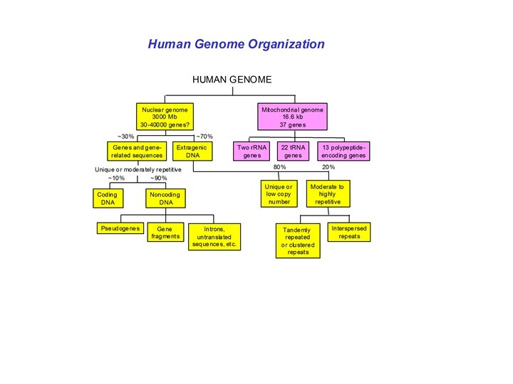
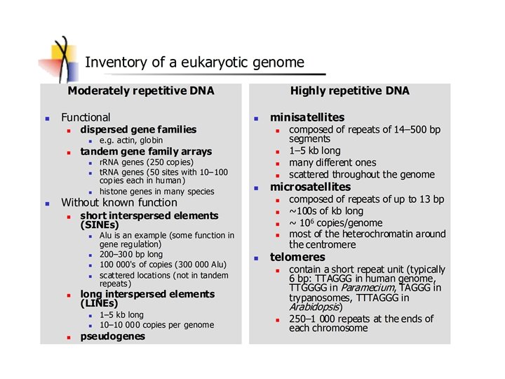
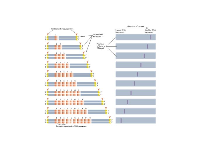
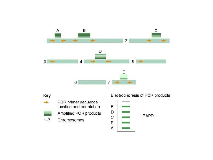
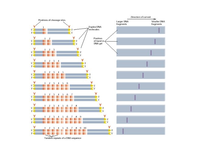
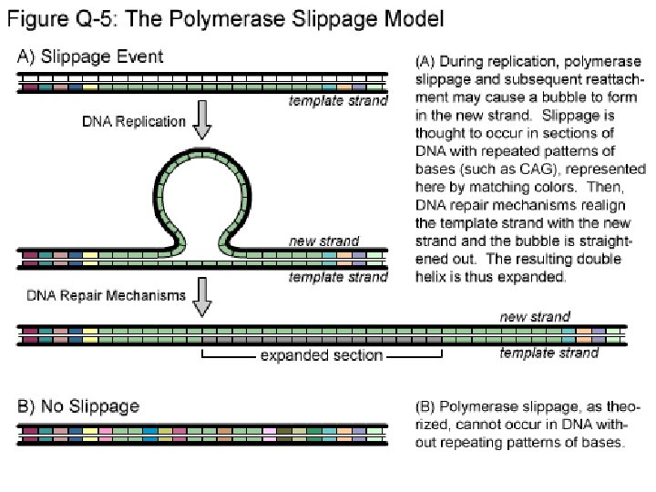
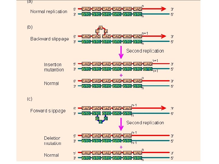
 VNTR: variable number of tandem repeats") Polymorphism induced by size variation (number of copies) VNTR: variable number of tandem repeats relatively small tandemly repeated sequences: dispersed in the genome e. g. minisatellites: repeat lengths of 10 -100’s of base pairs microsatellites: have repeated lengths of one or some base pairs RAPD: random amplified polymorphic DNA produces a large number of fragments, many species-specific if inheritance verified: RAPD patterns can be used in population genetics
Polymorphism induced by size variation (number of copies) VNTR: variable number of tandem repeats relatively small tandemly repeated sequences: dispersed in the genome e. g. minisatellites: repeat lengths of 10 -100’s of base pairs microsatellites: have repeated lengths of one or some base pairs RAPD: random amplified polymorphic DNA produces a large number of fragments, many species-specific if inheritance verified: RAPD patterns can be used in population genetics
 RAPD: Random Amplified Polymorphic DNA • PCR-based marker with 10 – 12 bp primers • Random amplification of several fragments • Amplified fragments run in a agarose gel and detected by ethidium bromide • Unstable amplification leads to poor repeatability
") PCR (Polymerase Chain Reaction)
PCR (Polymerase Chain Reaction)
 The mixture after the PCR reaction is normally loaded on an agarose gel for electrophoresis to separate amplification products according to their size. Staining of the gel with ethidium bromide, and subsequent observation under ultraviolet light is the next step. Ethidium bromide will concentrate between the bases in the DNA and give rise to yellow flourescent bands under the UV-light. The present RAPD reactions show amplification of nine different chromosome segments in the agarose gel. The B 3 band is polymorphic with a longer amplification product from L 1 than from L 2. Because both alleles can be seen in the F 1 this marker is codominant. The B 6 band is absent in the reaction from the line L 1, possibly because one of the primer sites has changed owing to a mutation. Dominant marker types are the most frequent in RAPD analysis.
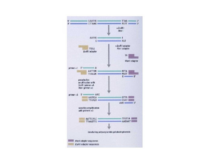
 AFLP: Amplified Fragment Length Polymorphism • Restriction endonuclease digestion of DNA (Eco. R i/Mse I, Eco. R i/Pst I) • Ligation of adapters • Amplification of the ligated fragments • Separation of the amplified fragments via electrophoresis and visualization • AFLPS have stable amplification and good repeatability • AFLPs may not be mapped and are technically difficult to perform
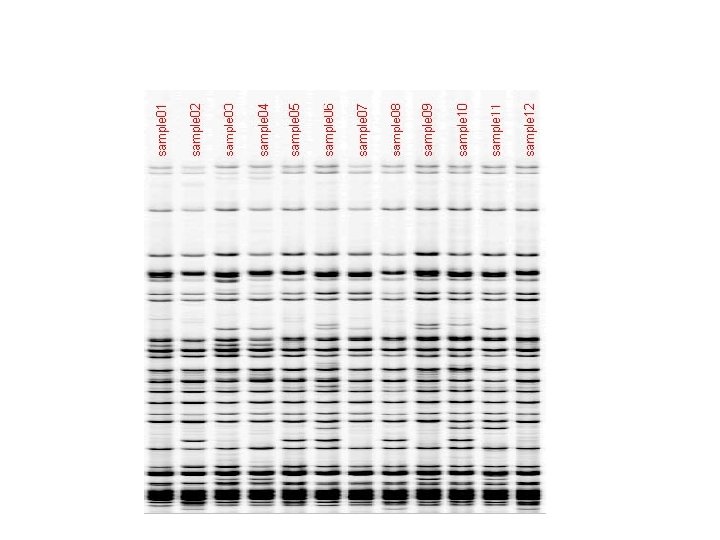
 AFLP reactions can be analysed by separation according to fragment size on a polyacrylamide gel. Visualisation is often done by autoradiography if one primer has P 33 labeling. The simplified autoradiograph from an AFLP (right) shows 27 different amplification products. The B 9 is a rare codominant marker with the fragment from line L 1 larger than the one form L 2. Both alleles are visible in the hybrid. B 18 and B 21 are of the much more frequent dominant types, where only one allele will amplify.
 SSR: Simple Sequence Repeat or Microsatellite • PCR-based marker with 18 -25 bp primers • SSR polymorphisms are based on number of repeat units, and are hypervariable (have many alleles) • Primers are mapped and reported in Maize. DB (www. agron. Missouri. edu/probes. Html) • SSRs have stable amplification and good repeatability • SSRs are easy to run and automate
 STS: Sequence Tagged Sites • PCR-based marker with 18 – 25 bp primers • Derived from sequenced RFLP, RAPD or AFLP fragments or known genes • Stable amplification and good repeatability • Generally mapped • Easy to run and automate • Not many polymorphic STSs currently available
 Species DNA Extraction Sequencing and primer design Clone Genotype analysis of fluorescent PCR Analysis of marker polymorphism atggctatcgattttgctatgc gagcggttaaaatctatgttgggat atggtatttgaatctcgtatcgctgta tcgctgatgcgcgcgcgcttatctgctatcgttsa gctatcgttcgggttaggtttatatgt agtctcgtcgctcatagttagctggt tatcttatcgtctcgatct Gel Electrophoresis PCR
 DNA sequencing: * sequencing: nucleotide sequences of DNA or RNA: greatest genotype resolution (looks at the nucleotide itself) - direct sequencing of genomic DNA (PCR) - or by cloning such regions and sequencing from the cloned fragment * nuclear genes: single locus nuclear genes detecting functional polymorphisms and population structure * mitochondrial DNA: cytoplasmic mt. DNA high number of copies, inherited from female parent, gives insight into sex-biased population structure, mt. DNA highly variable, classically used in population biology * transposons: polymorphism induced by insertion, horizontal gene transfer (transfer of DNA segments between organisms), inter-organellar gene transfer (between organelles within organisms)
 Choice of molecular markers to determine parentage depending on the level of evolutionary divergence most molecular markers: variation in noncoding DNA regions in general: allozymes less variable than RAPD or RFLP markers RAPD/RFLP markers less variable than micro/minisatellite fingerprints
 Definitions • Traits examined so far have resulted in discontinuous phenotypic traits – Tall or dwarf – Round or wrinkled – Red, pink or white • Most of phenotypic traits vary on a continuous basis: – Height – Weight – Fitness
 What is a Quantitative Trait? A quantitative trait has numerical values that can be ordered highest to lowest.
 Describing Quantitative Traits: The Mean • Two statistics are commonly used to describe variation of a quantitative trait in a population 1 The Mean - For a trait that forms a bell shaped curve (normal distribution) when a frequency diagram is plotted, the mean is the most common size, shape, or whatever is being measured SXi X= n Number of individual values X D Frequency Sum of individual values D Trait
 Describing Quantitative Traits: Standard Deviation 2 Standard Deviation - Describes the amount of variation from the mean in units of the trait • Large SD indicates great variability • 68 % of individuals exhibiting the trait will fall within ± 1 SD of the mean, 95. 5 % ± 2, 99. 7 % ± 3 SD • 95 % fall within 1. 96 SD -1 +1 D Frequency X 68. 3% D Trait
 DEVIAZIONE STANDARD VARIANZA
![COVARIANZA [COV X, Y] COEFFICIENTE DI CORRELAZIONE=r=](https://present5.com/presentation/5d728aef9882aa1228f56ffe0c9c8ed2/image-52.jpg "COVARIANZA [COV X, Y] COEFFICIENTE DI CORRELAZIONE=r=") COVARIANZA [COV X, Y] COEFFICIENTE DI CORRELAZIONE=r=
COVARIANZA [COV X, Y] COEFFICIENTE DI CORRELAZIONE=r=
![ANALISI DELLA REGRESSIONE Y=A + BX B=COV [X, Y] Varianza X](https://present5.com/presentation/5d728aef9882aa1228f56ffe0c9c8ed2/image-53.jpg "ANALISI DELLA REGRESSIONE Y=A + BX B=COV [X, Y] Varianza X") ANALISI DELLA REGRESSIONE Y=A + BX B=COV [X, Y] Varianza X
ANALISI DELLA REGRESSIONE Y=A + BX B=COV [X, Y] Varianza X
 Separating Genetics from Environment • Two experiments by Wilhelm Johannsen, from Denmark, using the common bean (Phaseolus vulgaris). Johannsen coined the words “genotype” and “phenotype”. • First Johannsen experiment: he weighed a group of beans, then grew them up and weighed their progeny (after selfing them).
 In general, heavy parents gave heavy offspring and light parents gave light offspring. That is, there is a significant correlation between parent and offspring weights. However, there is also a considerable variation among the offspring weights.
 Johannsen’s Second Experiment • Johannsen then worked on separating environmental effects from genetic effects. He did this by inbreeding the beans for 10 generations. . • After 10 generations of selfing, the percentage of heterozygotes is less than 1/1000 of the original level.
 Results • Johannsen created 19 inbred lines. The inbred lines had some variation, but less than the original randombred population. The remaining variation was due to environmental variations. • The mean weight of each line was different, but it was stable across generations. The reason is that the lines are genetically different from each other, but they are genetically (more or less) identical. The variance was also stable between generations.
 • • Start with a random-bred population. Take the best ones to be parents of the next generation. The next generation has a mean that is shifted in the desired direction. This procedure doesn’t work for inbred populations, because there is no genetic variation to inherit. The next generation’s mean is the same as the previous generation’s mean despite having selected the best parents.
 Mathematical Basis of Quantitative Genetics • • • Recall the basic premise of quantitative genetics: phenotype = genetics plus environment. In fact we are looking at variation in the traits, which is measured by the width of the Gaussian distribution curve. This width is the variance (or its square root, the standard deviation). Variance is a useful property, because variances from different sources can be added together to get total variance. However, the units of variance are the squares of the units used to measure the trait. Thus, if length in centimeters was measured, the variances of the length are in cm 2. This is why standard deviation is usually reported: length ± s. d. --because standard deviation is in the same units as the original measurement. Standard deviations from different sources are not additive. Quantitative traits can thus be expressed as: VT = V G + V E where VT = total variance, VG - variance due to genetics, and VE = variance due to environmental (non-inherited) causes. This equation is often written with an additional covariance term: the degree to which genetic and environmental variance depend on each other. We are just going to assume this term equals zero in our discussions.
 Heritability • One property of interest is “heritability”, the proportion of a trait’s variation that is due to genetics (with the rest of it due to “environmental” factors). This seems like a simple concept, but it is loaded with problems. • The broad-sense heritability, symbolized as H (sometimes H 2 to indicate that the units of variance are squared). H is a simple translation of the statement from above into mathematics: H = V G / VT • This measure, the broad-sense heritability, is fairly easy to measure, especially in human populations where identical twins are available. However, different studies show wide variations in H values for the same traits, and plant breeders have found that it doesn’t accurately reflect the results of selection experiments. Thus, H is generally only used in social science work.
 Additive vs. Dominance Genetic Variance • • • The biggest problem with broad sense heritability comes from lumping all genetic phenomena into a single Vg factor. Paradoxically, not all variation due to genetic differences can be directly inherited by an offspring from the parents. Genetic variance can be split into 2 main components, additive genetic variance (VA) and dominance genetic variance (VD). VG = V A + V D Additive variance is the variance in a trait that is due to the effects of each individual allele being added together, without any interactions with other alleles or genes. Dominance variance is the variance that is due to interactions between alleles: synergy, effects due to two alleles interacting to make the trait greater (or lesser) than the sum of the two alleles acting alone. We are using dominance variance to include both interactions between alleles of the same gene and interactions between difference genes, which is sometimes a separate component called epistasis variance. The important point: dominance variance is not directly inherited from parent to offspring. It is due to the interaction of genes from both parents within the individual, and of course only one allele is passed from each parent to the offspring.
 Narrow Sense Heritability • For a practical breeder, dominance variance can’t be predicted, and it doesn’t affect the mean or variance of the offspring of a selection cross in a systematic fashion. Thus, only additive genetic variance is useful. Breeders and other scientists use “narrow sense heritability”, h, as a measure of heritability. h = VA / VT • Narrow sense heritability can also be calculated directly from breeding experiments. For this reason it is also called “realized heritability”.
 Heritability in a Selection Experiment • There are 3 easily measured parameters in a selection experiment: the mean of the original random-bred population, the mean of the individuals selected to be the parents, and the mean of the next generation. These factors are related by the narrow sense heritability: • The denominator is sometimes called the “selection differential”, the difference between the total population and the individuals selected to be parents of the next generation. The numerator is sometimes called the “selection response”, the difference between the offspring and the original population, the amount the population shifted due to the selection.
 Example • In Drosophila, the mean number of bristles on the thorax (top surface only) is 6. 4. • From this population, a group was chosen which had an average bristle number of 7. 2. • The offspring of the chosen group had an average of 6. 6 bristles. • h = (next gen - original) / (selected - original) • h = (6. 6 - 6. 4) / (7. 2 - 6. 4) • h = 0. 2 / 0. 8 • h = 0. 25
 Example Problem • In a quest to make bigger frogs, scientists started with a random bred population of frogs with an average weight of 500 g. They chose a group with average weight 600 g to be the parents of the next generation. A few other facts: VE = 1340, VA = 870, VD = 410. • • • What is the genetic variance? VG = VA + VD = 1280 What is the total variance? VT = VG + VE = 2620 What is the broad sense heritability? H = VG / VT = 0. 49 What is the narrow sense heritability? h = VA / VT = 0. 33 What is the mean weight of the next generation? h = (next gen - original) / (selected - original) 0. 33 = (next_gen - 500) / (600 - 500) = 533 g
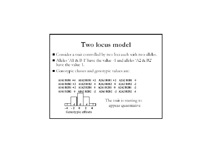
 Additive Alleles • If more than one gene with two alleles that behave as incompletely dominant alleles are involved, variability occurs over more of a continuum • If two genes with two alleles are involved, X phenotypes can result F 2 1/4 AA 1/2 Aa 1/4 aa Additive alleles 1/4 BB -- 1/16 AABB 4 1/2 Bb -- 2/16 AABb 3 1/4 bb -- 1/16 AAbb 2 1/4 BB -- 2/16 Aa. BB 3 1/2 Bb -- 4/16 Aa. Bb 2 1/4 bb -- 2/16 Aabb 1 1/4 BB -- 1/16 aa. BB 2 1/2 Bb -- 2/16 aa. Bb 1 1/4 bb -- 1/16 aabb 0 1/16 4/16 = 1/4 6/16 = 3/8 4/16 = 1/4 1/16
 Additive Alleles • Additive alleles are alleles that change the phenotype in an additive way • Example - The more copies of tall alleles a person has, the greater their potential for growing tall • Additive alleles behave something like alleles that result in incomplete dominance • More CR alleles results in F 2 Generation redder flowers CR CW C RC R C RC W 1: R R 2: R W 1 W CW CRCW CWCW W
 Estimating Gene Numbers • The more genes involved in producing a trait, the more gradations will be observed in that trait • If two examples of extremes of variation for a trait are crossed and the F 2 progeny are examined, the proportion exhibiting the extreme variations can be used to calculate the number of genes involved: 1 = F extreme phenotypes in total offspring 2 4 n • If 1/64 th of the offspring of an F 2 cross of the kind described above are the same as the parents, then 1 = 1 N = 3 so there are probably 64 43 about 3 genes involved