EF 507 QUANTITATIVE METHODS FOR ECONOMICS AND FINANCE

EF 507 QUANTITATIVE METHODS FOR ECONOMICS AND FINANCE FALL 2008 Chapter 5 Discrete Random Variables and Probability Distributions Chap 5 -1

2

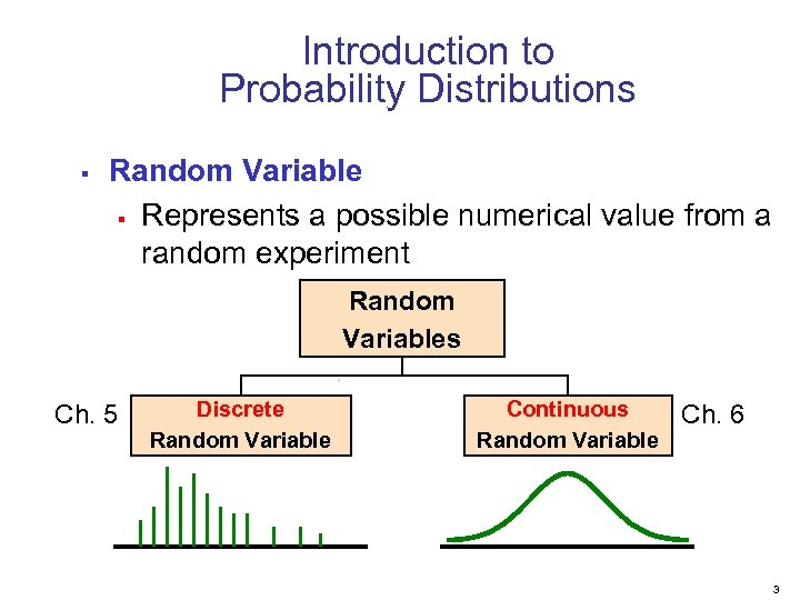Introduction to Probability Distributions § Random Variable § Represents a possible numerical value from a random experiment Random Variables Ch. 5 Discrete Random Variable Continuous Random Variable Ch. 6 3

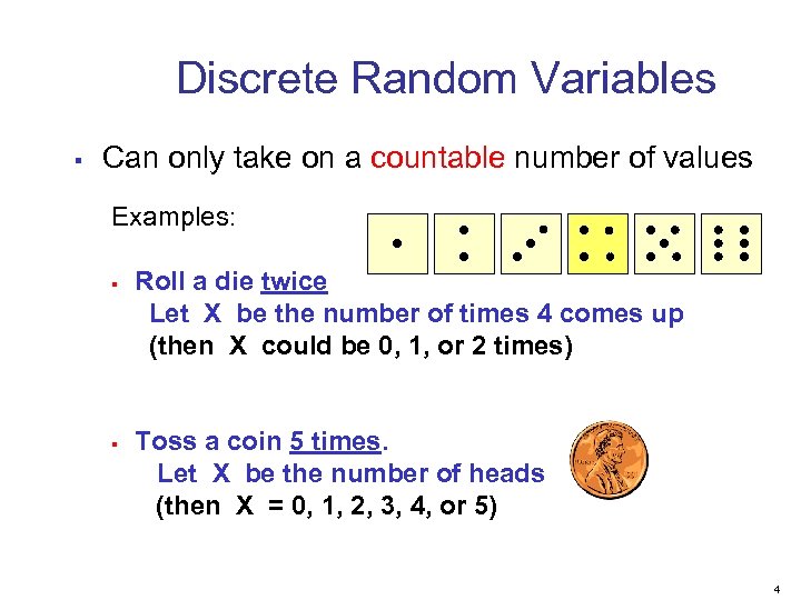Discrete Random Variables § Can only take on a countable number of values Examples: § § Roll a die twice Let X be the number of times 4 comes up (then X could be 0, 1, or 2 times) Toss a coin 5 times. Let X be the number of heads (then X = 0, 1, 2, 3, 4, or 5) 4

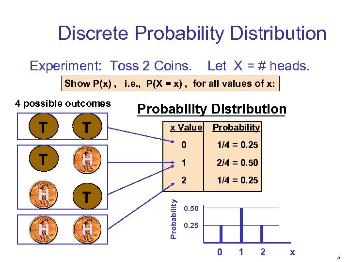Discrete Probability Distribution Experiment: Toss 2 Coins. Let X = # heads. Show P(x) , i. e. , P(X = x) , for all values of x: 4 possible outcomes T T Probability Distribution 1 2/4 = 0. 50 1/4 = 0. 25 H T H Probability H 1/4 = 0. 25 2 H Probability 0 T x Value 0. 50 0. 25 0 1 2 x 5

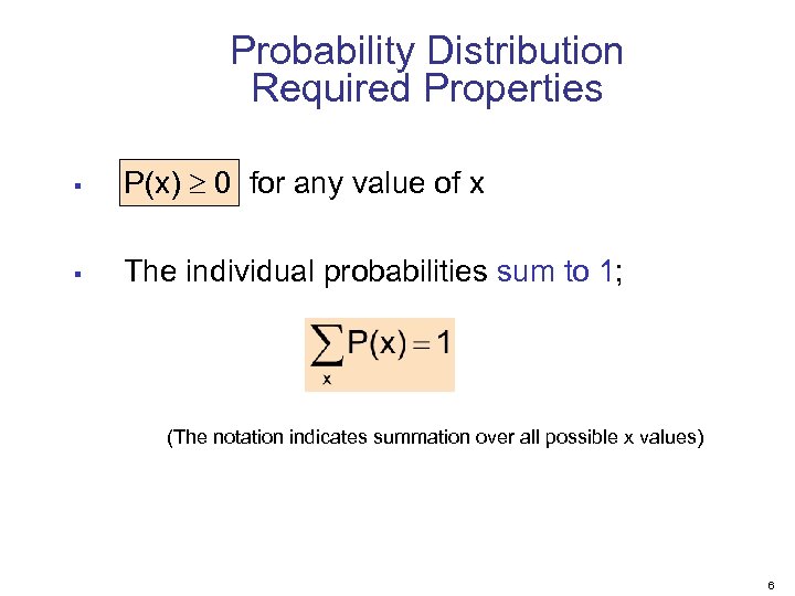Probability Distribution Required Properties § P(x) 0 for any value of x § The individual probabilities sum to 1; (The notation indicates summation over all possible x values) 6

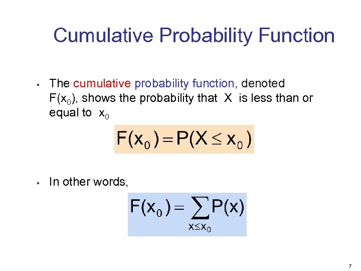Cumulative Probability Function § § The cumulative probability function, denoted F(x 0), shows the probability that X is less than or equal to x 0 In other words, 7

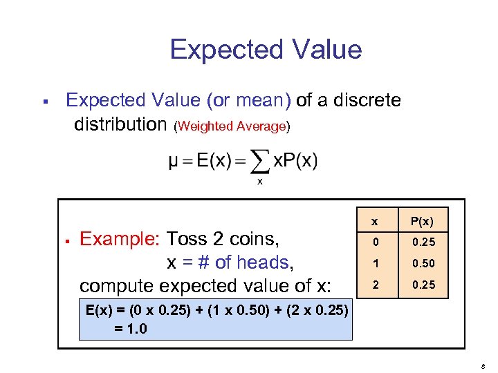Expected Value § Expected Value (or mean) of a discrete distribution (Weighted Average) x § Example: Toss 2 coins, x = # of heads, compute expected value of x: P(x) 0 0. 25 1 0. 50 2 0. 25 E(x) = (0 x 0. 25) + (1 x 0. 50) + (2 x 0. 25) = 1. 0 8

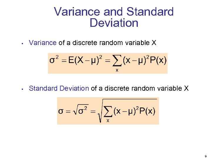Variance and Standard Deviation § Variance of a discrete random variable X § Standard Deviation of a discrete random variable X 9

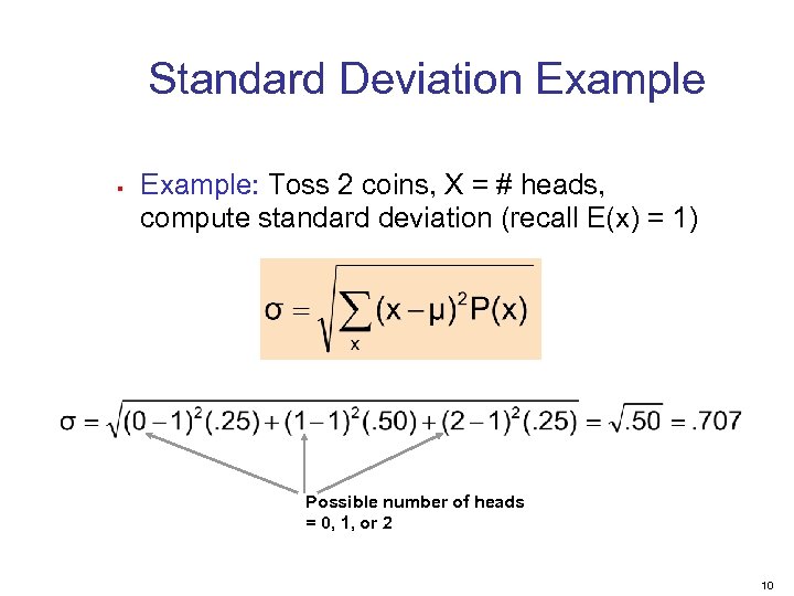Standard Deviation Example § Example: Toss 2 coins, X = # heads, compute standard deviation (recall E(x) = 1) Possible number of heads = 0, 1, or 2 10

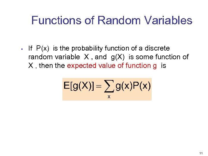Functions of Random Variables § If P(x) is the probability function of a discrete random variable X , and g(X) is some function of X , then the expected value of function g is 11

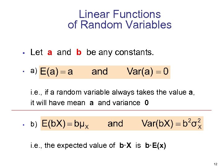Linear Functions of Random Variables § Let a and b be any constants. § a) i. e. , if a random variable always takes the value a, it will have mean a and variance 0 § b) i. e. , the expected value of b·X is b·E(x) 12

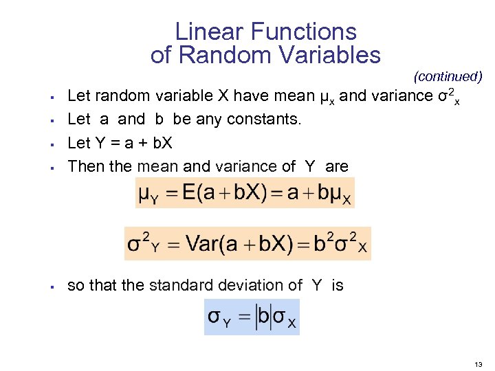Linear Functions of Random Variables (continued) § Let random variable X have mean µx and variance σ2 x Let a and b be any constants. Let Y = a + b. X Then the mean and variance of Y are § so that the standard deviation of Y is § § § 13

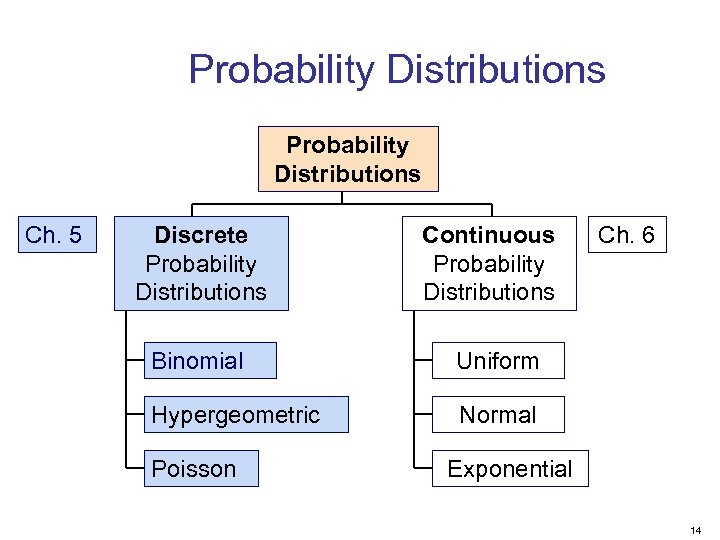Probability Distributions Ch. 5 Discrete Probability Distributions Continuous Probability Distributions Binomial Uniform Hypergeometric Ch. 6 Normal Poisson Exponential 14

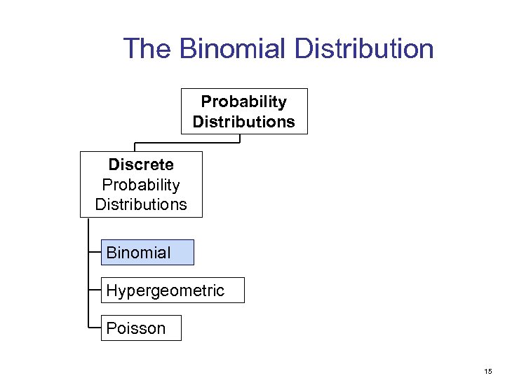The Binomial Distribution Probability Distributions Discrete Probability Distributions Binomial Hypergeometric Poisson 15

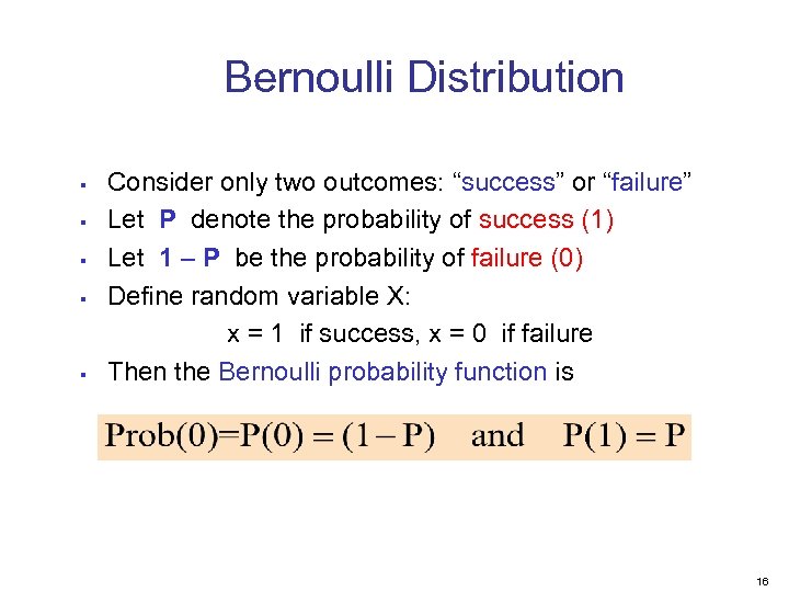Bernoulli Distribution § § § Consider only two outcomes: “success” or “failure” Let P denote the probability of success (1) Let 1 – P be the probability of failure (0) Define random variable X: x = 1 if success, x = 0 if failure Then the Bernoulli probability function is 16

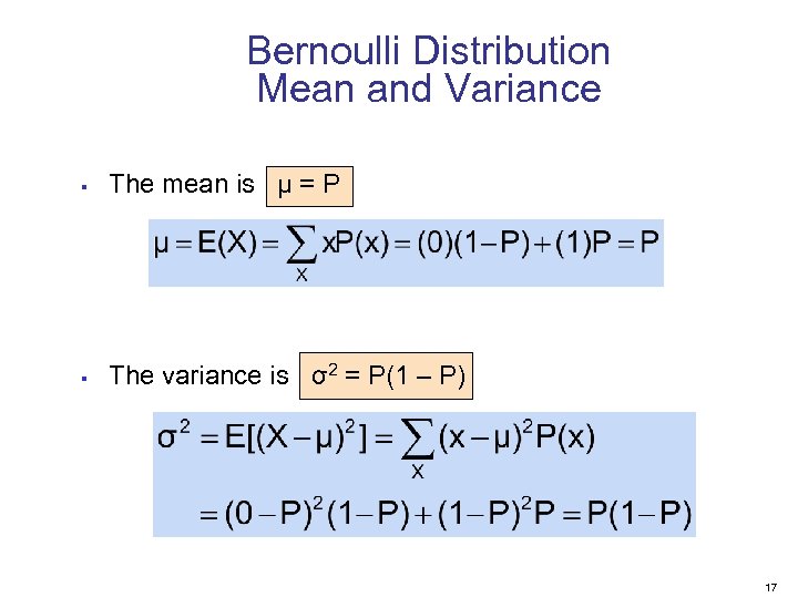Bernoulli Distribution Mean and Variance § The mean is µ = P § The variance is σ2 = P(1 – P) 17

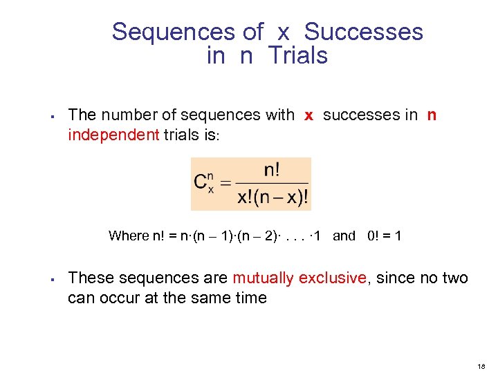Sequences of x Successes in n Trials § The number of sequences with x successes in n independent trials is: Where n! = n·(n – 1)·(n – 2)·. . . · 1 and 0! = 1 § These sequences are mutually exclusive, since no two can occur at the same time 18

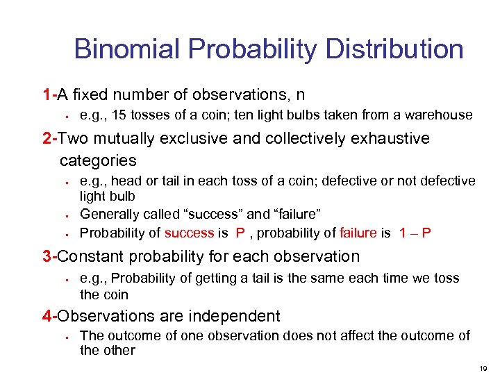Binomial Probability Distribution 1 -A fixed number of observations, n § e. g. , 15 tosses of a coin; ten light bulbs taken from a warehouse 2 -Two mutually exclusive and collectively exhaustive categories § § § e. g. , head or tail in each toss of a coin; defective or not defective light bulb Generally called “success” and “failure” Probability of success is P , probability of failure is 1 – P 3 -Constant probability for each observation § e. g. , Probability of getting a tail is the same each time we toss the coin 4 -Observations are independent § The outcome of one observation does not affect the outcome of the other 19

Possible Binomial Distribution Settings § § A manufacturing plant labels items as either defective or acceptable A firm bidding for contracts will either get a contract or not A marketing research firm receives survey responses of “Yes I will buy” or “No I will not” New job applicants either accept the offer or reject it 20

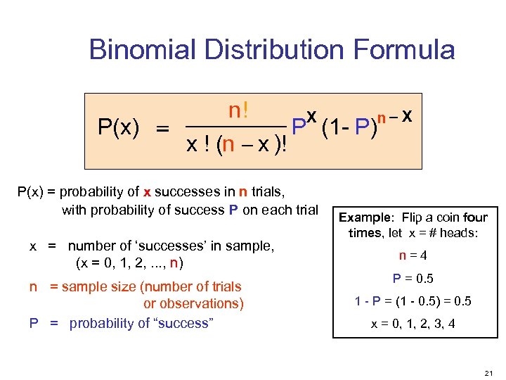Binomial Distribution Formula P(x) = n! x ! (n - x )! X P (1 - P) P(x) = probability of x successes in n trials, with probability of success P on each trial x = number of ‘successes’ in sample, (x = 0, 1, 2, . . . , n) n = sample size (number of trials or observations) P = probability of “success” n-X Example: Flip a coin four times, let x = # heads: n=4 P = 0. 5 1 - P = (1 - 0. 5) = 0. 5 x = 0, 1, 2, 3, 4 21

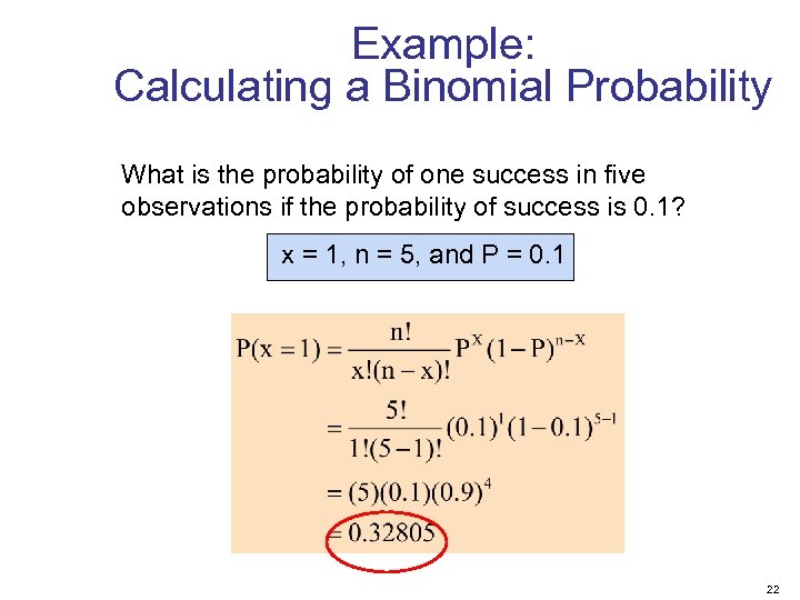Example: Calculating a Binomial Probability What is the probability of one success in five observations if the probability of success is 0. 1? x = 1, n = 5, and P = 0. 1 22

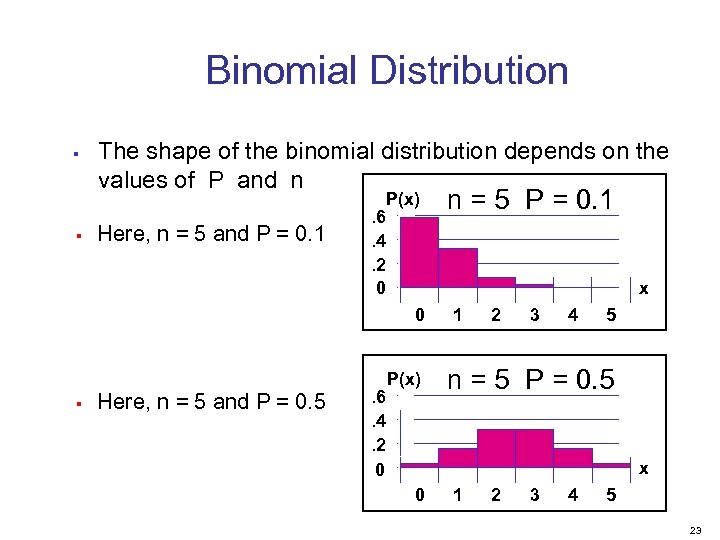Binomial Distribution § The shape of the binomial distribution depends on the values of P and n Mean § Here, n = 5 and P = 0. 1 . 6. 4. 2 0 P(x) x 0 § Here, n = 5 and P = 0. 5 . 6. 4. 2 0 n = 5 P = 0. 1 P(x) 1 2 3 4 5 n = 5 P = 0. 5 x 0 1 2 3 4 5 23

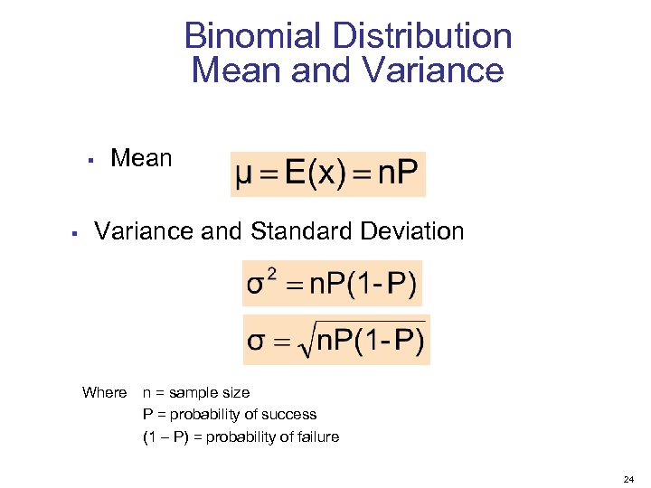Binomial Distribution Mean and Variance § § Mean Variance and Standard Deviation Where n = sample size P = probability of success (1 – P) = probability of failure 24

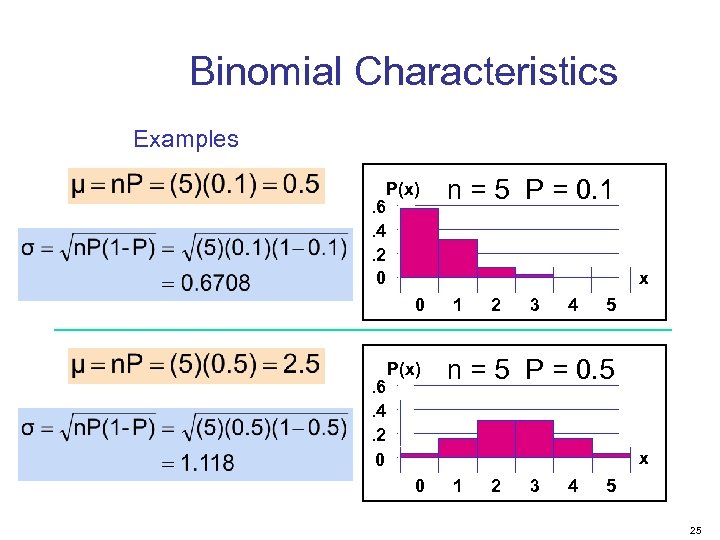Binomial Characteristics Examples Mean . 6. 4. 2 0 P(x) x 0 . 6. 4. 2 0 n = 5 P = 0. 1 P(x) 1 2 3 4 5 n = 5 P = 0. 5 x 0 1 2 3 4 5 25

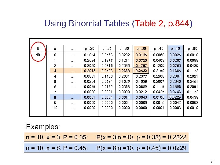Using Binomial Tables (Table 2, p. 844) N x … p=. 20 p=. 25 p=. 30 p=. 35 p=. 40 p=. 45 p=. 50 10 0 1 2 3 4 5 6 7 8 9 10 … … … 0. 1074 0. 2684 0. 3020 0. 2013 0. 0881 0. 0264 0. 0055 0. 0008 0. 0001 0. 0000 0. 0563 0. 1877 0. 2816 0. 2503 0. 1460 0. 0584 0. 0162 0. 0031 0. 0004 0. 0000 0. 0282 0. 1211 0. 2335 0. 2668 0. 2001 0. 1029 0. 0368 0. 0090 0. 0014 0. 0001 0. 0000 0. 0135 0. 0725 0. 1757 0. 2522 0. 2377 0. 1536 0. 0689 0. 0212 0. 0043 0. 0005 0. 0000 0. 0060 0. 0403 0. 1209 0. 2150 0. 2508 0. 2007 0. 1115 0. 0425 0. 0106 0. 0016 0. 0001 0. 0025 0. 0207 0. 0763 0. 1665 0. 2384 0. 2340 0. 1596 0. 0746 0. 0229 0. 0042 0. 0003 0. 0010 0. 0098 0. 0439 0. 1172 0. 2051 0. 2461 0. 2051 0. 1172 0. 0439 0. 0098 0. 0010 Examples: n = 10, x = 3, P = 0. 35: P(x = 3|n =10, p = 0. 35) = 0. 2522 n = 10, x = 8, P = 0. 45: P(x = 8|n =10, p = 0. 45) = 0. 0229 26

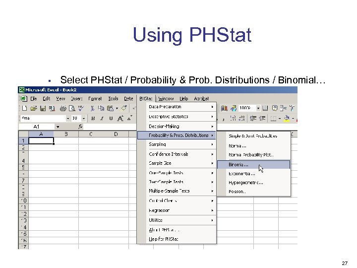Using PHStat § Select PHStat / Probability & Prob. Distributions / Binomial… 27

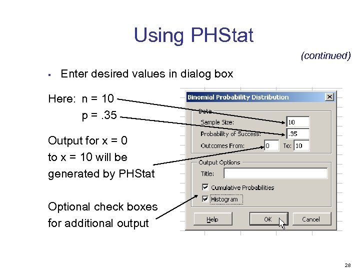Using PHStat (continued) § Enter desired values in dialog box Here: n = 10 p =. 35 Output for x = 0 to x = 10 will be generated by PHStat Optional check boxes for additional output 28

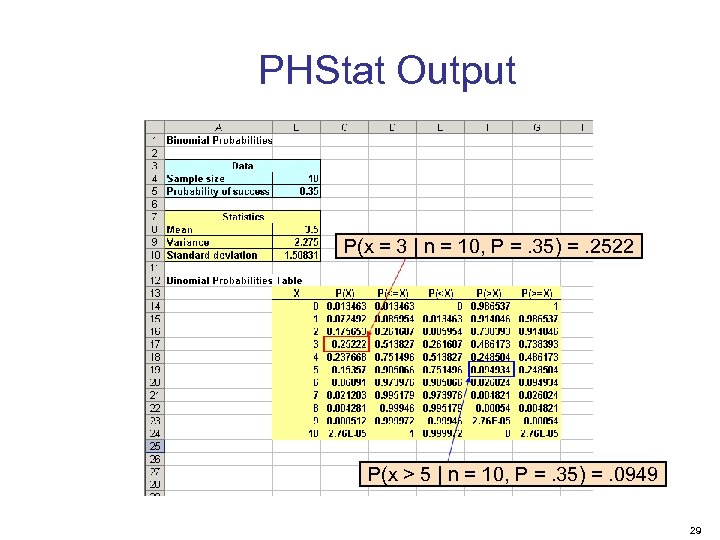PHStat Output P(x = 3 | n = 10, P =. 35) =. 2522 P(x > 5 | n = 10, P =. 35) =. 0949 29

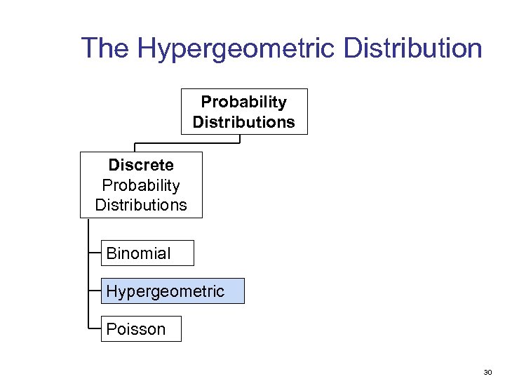The Hypergeometric Distribution Probability Distributions Discrete Probability Distributions Binomial Hypergeometric Poisson 30

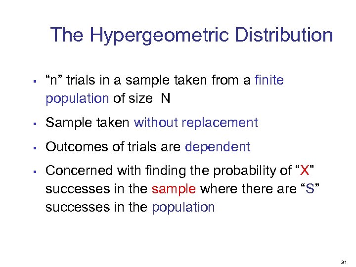The Hypergeometric Distribution § “n” trials in a sample taken from a finite population of size N § Sample taken without replacement § Outcomes of trials are dependent § Concerned with finding the probability of “X” successes in the sample where there are “S” successes in the population 31

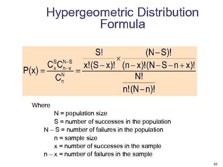Hypergeometric Distribution Formula Where N = population size S = number of successes in the population N – S = number of failures in the population n = sample size x = number of successes in the sample n – x = number of failures in the sample 32

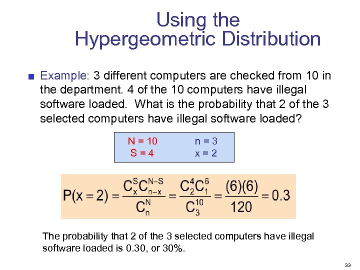Using the Hypergeometric Distribution ■ Example: 3 different computers are checked from 10 in the department. 4 of the 10 computers have illegal software loaded. What is the probability that 2 of the 3 selected computers have illegal software loaded? N = 10 S=4 n=3 x=2 The probability that 2 of the 3 selected computers have illegal software loaded is 0. 30, or 30%. 33

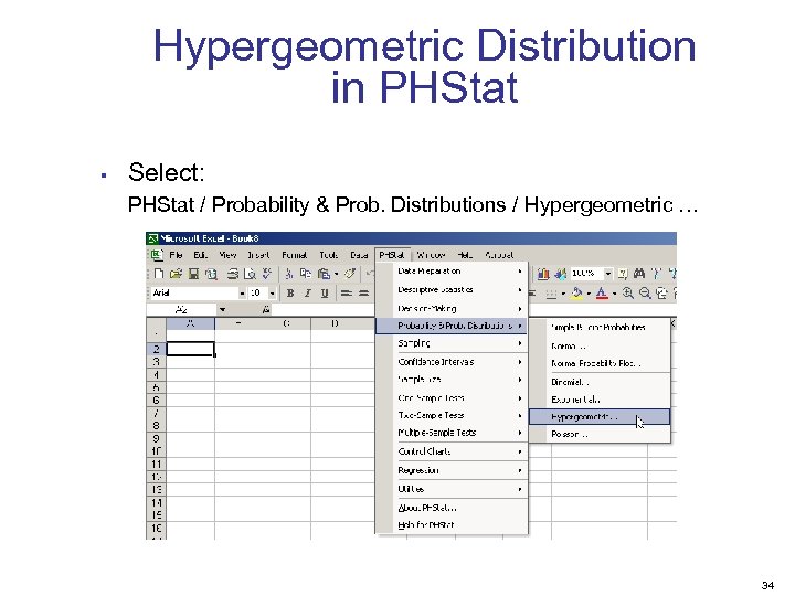Hypergeometric Distribution in PHStat § Select: PHStat / Probability & Prob. Distributions / Hypergeometric … 34

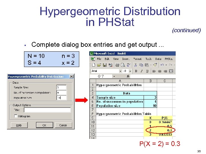Hypergeometric Distribution in PHStat (continued) § Complete dialog box entries and get output … N = 10 S=4 n=3 x=2 P(X = 2) = 0. 3 35

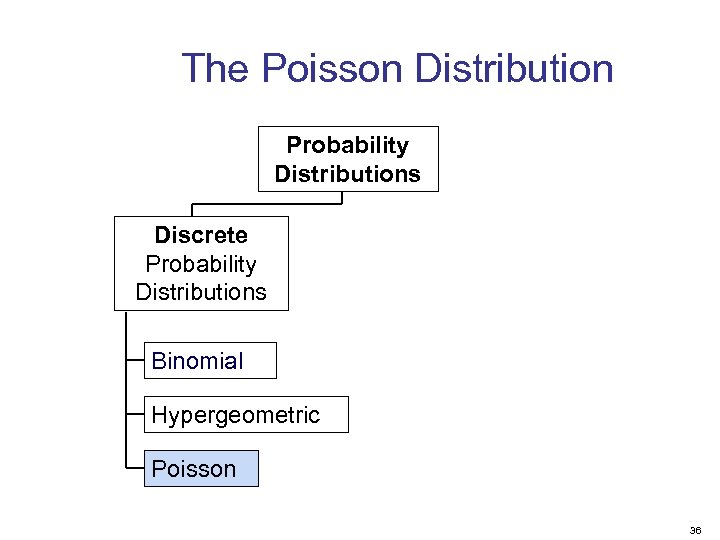The Poisson Distribution Probability Distributions Discrete Probability Distributions Binomial Hypergeometric Poisson 36

The Poisson Distribution § Apply the Poisson Distribution when: 1 -You wish to count the number of times an event occurs in a given continuous interval 2 -The probability that an event occurs in one subinterval is very small and is the same for all subintervals 3 -The number of events that occur in one subinterval is independent of the number of events that occur in the other subintervals 4 -There can be no more than one occurrence in each subinterval 5 -The average number of events per unit is (lambda) 37

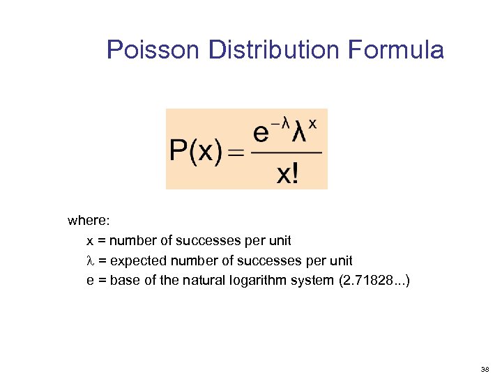Poisson Distribution Formula where: x = number of successes per unit = expected number of successes per unit e = base of the natural logarithm system (2. 71828. . . ) 38

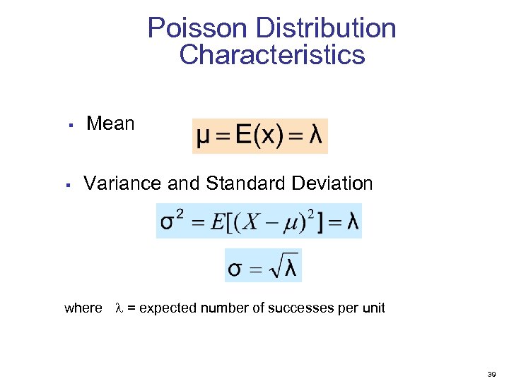Poisson Distribution Characteristics § Mean § Variance and Standard Deviation where = expected number of successes per unit 39

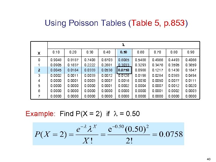Using Poisson Tables (Table 5, p. 853) X 0. 10 0. 20 0. 30 0. 40 0. 50 0. 60 0. 70 0. 80 0. 90 0 1 2 3 4 5 6 7 0. 9048 0. 0905 0. 0045 0. 0002 0. 0000 0. 8187 0. 1637 0. 0164 0. 0011 0. 0000 0. 7408 0. 2222 0. 0333 0. 0003 0. 0000 0. 6703 0. 2681 0. 0536 0. 0072 0. 0007 0. 0001 0. 0000 0. 6065 0. 3033 0. 0758 0. 0126 0. 0016 0. 0002 0. 0000 0. 5488 0. 3293 0. 0988 0. 0198 0. 0030 0. 0004 0. 0000 0. 4966 0. 3476 0. 1217 0. 0284 0. 0050 0. 0007 0. 0001 0. 0000 0. 4493 0. 3595 0. 1438 0. 0383 0. 0077 0. 0012 0. 0000 0. 4066 0. 3659 0. 1647 0. 0494 0. 0111 0. 0020 0. 0003 0. 0000 Example: Find P(X = 2) if = 0. 50 40

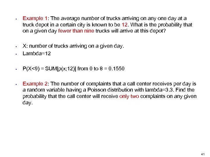§ Example 1: The average number of trucks arriving on any one day at a truck depot in a certain city is known to be 12. What is the probability that on a given day fewer than nine trucks will arrive at this depot? § X: number of trucks arriving on a given day. Lambda=12 § P(X<9) = SUM[p(x; 12)] from 0 to 8 = 0. 1550 § § Example 2: The number of complaints that a call center receives per day is a random variable having a Poisson distribution with lambda=3. 3. Find the probability that the call center will receive only two complaints on any given day. 41

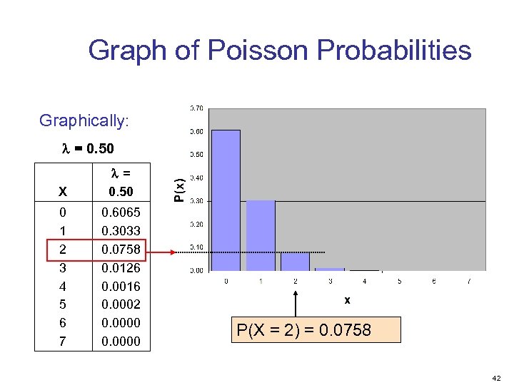Graph of Poisson Probabilities Graphically: = 0. 50 X = 0. 50 0 1 2 3 4 5 6 7 0. 6065 0. 3033 0. 0758 0. 0126 0. 0016 0. 0002 0. 0000 P(X = 2) = 0. 0758 42

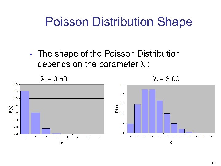Poisson Distribution Shape § The shape of the Poisson Distribution depends on the parameter : = 0. 50 = 3. 00 43

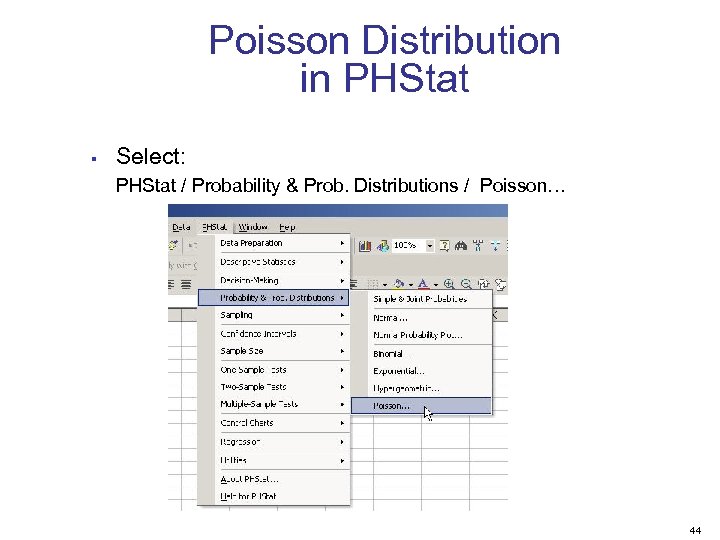Poisson Distribution in PHStat § Select: PHStat / Probability & Prob. Distributions / Poisson… 44

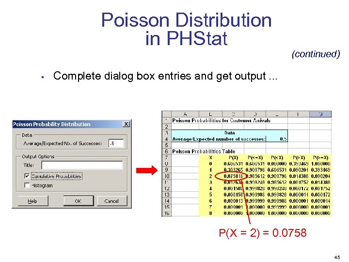Poisson Distribution in PHStat § (continued) Complete dialog box entries and get output … P(X = 2) = 0. 0758 45

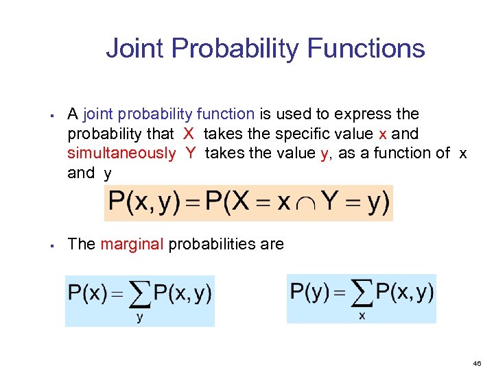Joint Probability Functions § § A joint probability function is used to express the probability that X takes the specific value x and simultaneously Y takes the value y, as a function of x and y The marginal probabilities are 46

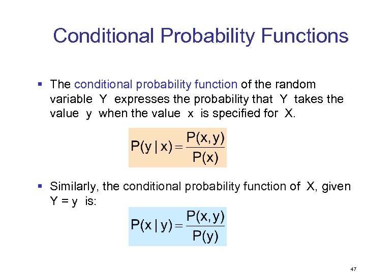Conditional Probability Functions § The conditional probability function of the random variable Y expresses the probability that Y takes the value y when the value x is specified for X. § Similarly, the conditional probability function of X, given Y = y is: 47

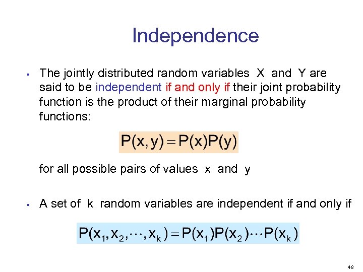Independence § The jointly distributed random variables X and Y are said to be independent if and only if their joint probability function is the product of their marginal probability functions: for all possible pairs of values x and y § A set of k random variables are independent if and only if 48

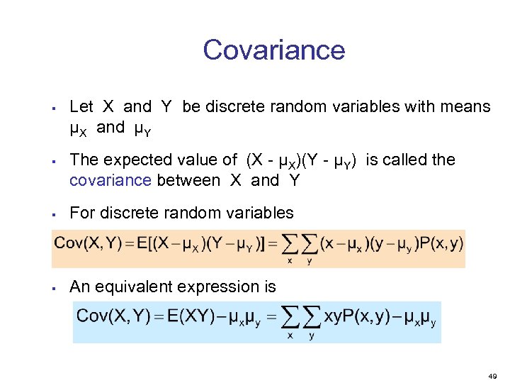Covariance § § Let X and Y be discrete random variables with means μX and μY The expected value of (X - μX)(Y - μY) is called the covariance between X and Y § For discrete random variables § An equivalent expression is 49

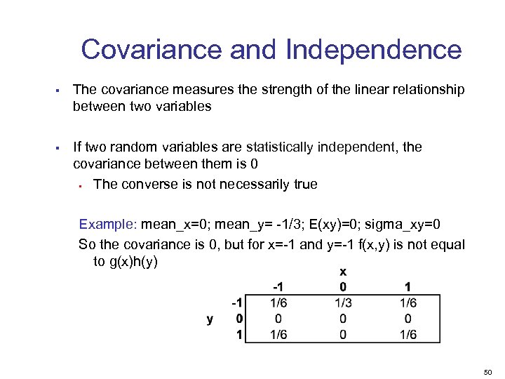Covariance and Independence § § The covariance measures the strength of the linear relationship between two variables If two random variables are statistically independent, the covariance between them is 0 § The converse is not necessarily true Example: mean_x=0; mean_y= -1/3; E(xy)=0; sigma_xy=0 So the covariance is 0, but for x=-1 and y=-1 f(x, y) is not equal to g(x)h(y) 50

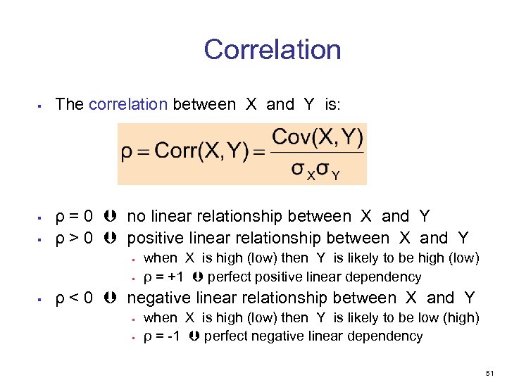Correlation § § § The correlation between X and Y is: ρ = 0 no linear relationship between X and Y ρ > 0 positive linear relationship between X and Y § § § when X is high (low) then Y is likely to be high (low) ρ = +1 perfect positive linear dependency ρ < 0 negative linear relationship between X and Y § § when X is high (low) then Y is likely to be low (high) ρ = -1 perfect negative linear dependency 51

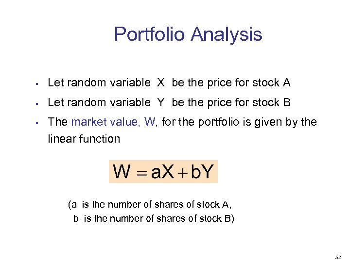Portfolio Analysis § Let random variable X be the price for stock A § Let random variable Y be the price for stock B § The market value, W, for the portfolio is given by the linear function (a is the number of shares of stock A, b is the number of shares of stock B) 52

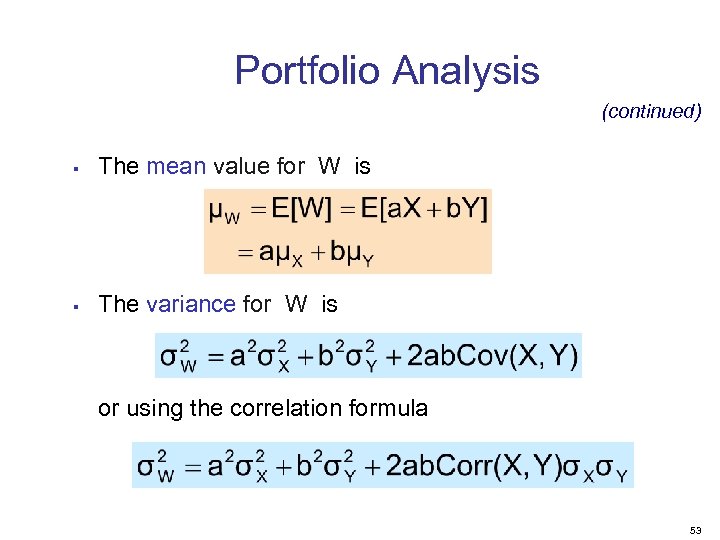Portfolio Analysis (continued) § The mean value for W is § The variance for W is or using the correlation formula 53

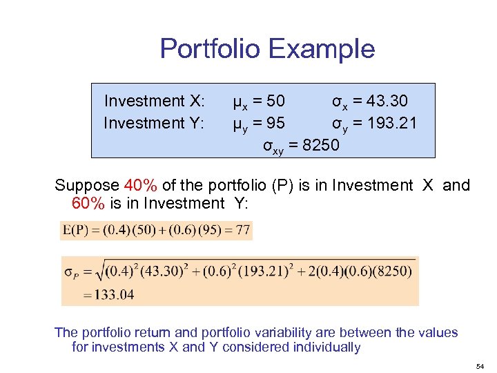Portfolio Example Investment X: Investment Y: μx = 50 σx = 43. 30 μy = 95 σy = 193. 21 σxy = 8250 Suppose 40% of the portfolio (P) is in Investment X and 60% is in Investment Y: The portfolio return and portfolio variability are between the values for investments X and Y considered individually 54

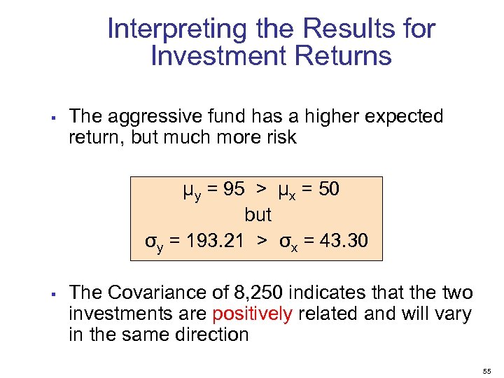Interpreting the Results for Investment Returns § The aggressive fund has a higher expected return, but much more risk μy = 95 > μx = 50 but σy = 193. 21 > σx = 43. 30 § The Covariance of 8, 250 indicates that the two investments are positively related and will vary in the same direction 55

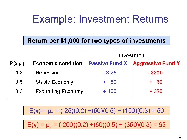Example: Investment Returns Return per $1, 000 for two types of investments P(xiyi) Economic condition Investment Passive Fund X Aggressive Fund Y 0. 2 Recession - $ 25 - $200 0. 5 Stable Economy + 50 + 60 0. 3 Expanding Economy + 100 + 350 E(x) = μx = (-25)(0. 2) +(50)(0. 5) + (100)(0. 3) = 50 E(y) = μy = (-200)(0. 2) +(60)(0. 5) + (350)(0. 3) = 95 56

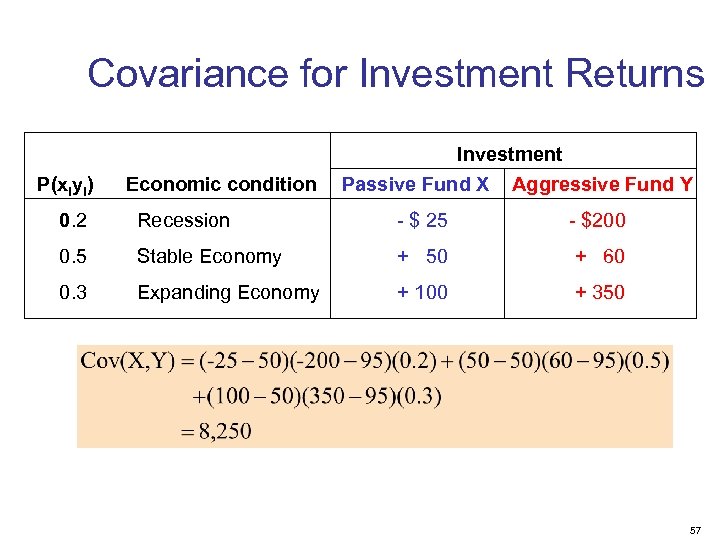Covariance for Investment Returns P(xiyi) Economic condition Investment Passive Fund X Aggressive Fund Y 0. 2 Recession - $ 25 - $200 0. 5 Stable Economy + 50 + 60 0. 3 Expanding Economy + 100 + 350 57

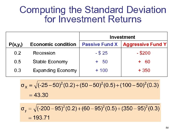Computing the Standard Deviation for Investment Returns P(xiyi) Economic condition Investment Passive Fund X Aggressive Fund Y 0. 2 Recession - $ 25 - $200 0. 5 Stable Economy + 50 + 60 0. 3 Expanding Economy + 100 + 350 58