

544815a513396f4376927ce1989a2791.ppt
- Количество слайдов: 73
 ECONOMICS what is it and why study it? Social Science Efficiency
 How to increase output • Economic Resources – Anything that can be used to produce output can be viewed as a resource (input, or factor of production) – Main categories of resources: • Land (inclusive of natural resources) • Physical Capital (productive capital) – Encouragement of saving (IRAs) • Labor – Immigration • Human Capital – Subsidized education • Entrepreneurship – Development of favorable business environment
 efficiency Output can be increased through increases in the resource base, but it can also be increased or “improved” through efficiency • Fundamental Economic Questions: – What to Produce (allocative efficiency) – How to Produce (productive efficiency) – For Whom to Produce (allocative efficiency) • The Society answers these questions in large part through the choice of the economic system
 Economic systems • Capitalism • Socialism • Communism These systems differ in the allocation of the ownership of productive resources The differences in these systems can also be formulated in terms of how they address the fundamental questions (e. g. command economy versus market economy) • Feudalism • Mercantilism
 Capitalism – Natural emergence • Adam Smith’s “invisible hand” concept – Simplified role of the government • Institutional support for economic activity – Property rights laws – Stable political system – Well defined legal system – Transparent business regulations – System of checks and balances for gov’t officials
 Socialism • Philosophical Foundation • Socialist Movement of the mid XIX century • Role of the government – Includes economic decisions in terms of allocation of resources and output, and possibly production
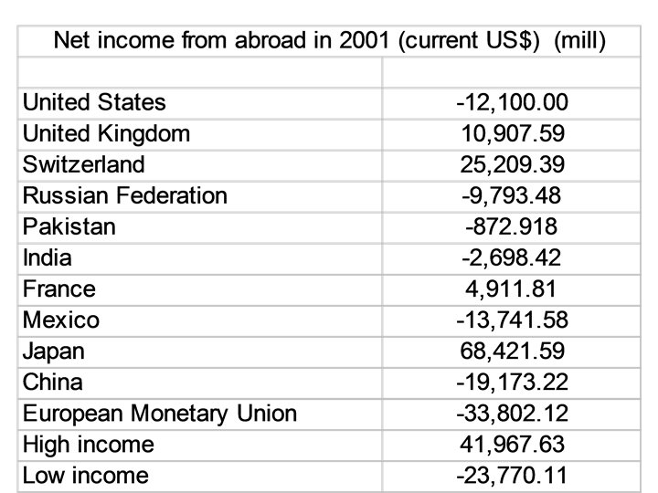
 – EU versus US versus RU") Modern Economies • Mixed system (capitalism + socialism) – EU versus US versus RU versus China General government final consumption expenditure (% of GDP) in 2001 Switzerland 13. 31 China 13. 69 United States 14. 23 Russian Federation 14. 32 Italy 18. 47 Germany 19. 06 France 23. 27 Sweden 26. 66 Source: World Bank, WDI 2003
Modern Economies • Mixed system (capitalism + socialism) – EU versus US versus RU versus China General government final consumption expenditure (% of GDP) in 2001 Switzerland 13. 31 China 13. 69 United States 14. 23 Russian Federation 14. 32 Italy 18. 47 Germany 19. 06 France 23. 27 Sweden 26. 66 Source: World Bank, WDI 2003
, 2000 Switzerland 2. 7") Unemployment rate comparison Unemployment, total (% of total labor force), 2000 Switzerland 2. 7 China 3. 1 United States 4. 1 Sweden 5. 1 Germany 8. 1 France 10. 0 Italy 10. 8 Russian Source: World Bank, WDI 2003 Federation 11. 4
Unemployment rate comparison Unemployment, total (% of total labor force), 2000 Switzerland 2. 7 China 3. 1 United States 4. 1 Sweden 5. 1 Germany 8. 1 France 10. 0 Italy 10. 8 Russian Source: World Bank, WDI 2003 Federation 11. 4
 The Concept of Cost in Economics • Every undertaken activity has a foregone sacrifice associated with it • Opportunity Cost – The value of the next BEST (highest valued) alternative (the value of the sacrifice that would have become the next choice) – E. g. opportunity cost of this class – E. g. Opportunity cost of the Colander’s book (relative price) – E. g. Opportunity cost of physical capital
 The world of trade-offs • Budget Constraint and Relative Price • Production Possibilities Frontier
 Gains from Trade • Specialization and increased output • Two-country two-product world • Absolute advantage principle – Why specialize in the production of something that is cheaper to purchase from abroad? • Comparative advantage principle – Specialize in the production of those products in which you have the lowest relative (opportunity) cost of production • Shape of PPF and lack of complete specialization • US trade data available on BEA website at: http: //www. bea. gov/bea/di/home/trade. htm
 Share of US exports for top US trading partners Source: GSU Economic Forecasting Center
 – Geographical boundaries (internet,") Markets • Defining a market – Product definition (and competition) – Geographical boundaries (internet, shipping cost reduction – globalization and outsourcing) • Market forces: Buyers (demand) versus Sellers (supply) – Price and quantity as the outcome
Markets • Defining a market – Product definition (and competition) – Geographical boundaries (internet, shipping cost reduction – globalization and outsourcing) • Market forces: Buyers (demand) versus Sellers (supply) – Price and quantity as the outcome
 • Price and the Law of") demand • Quantity = f (price, other factors) • Price and the Law of Demand • Other factors – Income (normal versus inferior) – Related in consumption goods • Substitutes • Complements – Expectations about the future – OTHER FACTORS ………
demand • Quantity = f (price, other factors) • Price and the Law of Demand • Other factors – Income (normal versus inferior) – Related in consumption goods • Substitutes • Complements – Expectations about the future – OTHER FACTORS ………
 • Price and the Law") supply • Quantity = f ( price, other factors) • Price and the Law of Supply • Other factors – Costs of Production (MC, and price as MB) – Goods related in production • Substitutes: (agricultural products) – Note, identical to costs of production since is based on opportunity cost concept • Complements: (like gold and silver) – Producer expectations of future prices • Other factors…
supply • Quantity = f ( price, other factors) • Price and the Law of Supply • Other factors – Costs of Production (MC, and price as MB) – Goods related in production • Substitutes: (agricultural products) – Note, identical to costs of production since is based on opportunity cost concept • Complements: (like gold and silver) – Producer expectations of future prices • Other factors…
 Market equilibrium • Qs = Qd • Shortage and surplus as unstable states and the stability property of the equilibrium • Market efficiency • Shifts in demand supply • Is the equilibrium really efficient? – Productive and allocative efficiency
 Market example: For. Ex • How can the US run a trade deficit consistently? Or, differently put, can one live on credit forever?
 Demand for the dollar different economic agents that purchase the dollar: • Foreigners who wish to purchase US goods or services, foreign tourists who wish to travel to the US (US exports) • Foreigners who wish to invest in the US (higher US interest rate, attractive US stock market returns) Supply of the dollar different economic agents that sell the dollar: • US consumers/firms that want to purchase foreign goods or services, US tourists who wish to travel abroad (US imports) • US residents who wish to invest abroad (higher interest rates abroad, etc. ) The dollar will appreciate if demand exceeds supply at the current exchange rate. Note that when you purchase a foreign made product, the cost of the production of that product is paid in foreign currency, hence somewhere between the production process and your purchase someone would have to convert your currency into that foreign currency in order to pay for the production.
 Demand supply: the USD • US trade deficit -> sale of USD ->dollar depreciation • US borrowing from abroad -> purchases of USD -> appreciation of the USD • 1990’s and the post 9/11 framework • US balance of payments: BEA
 Measuring Economic Activity • OUTPUT • EMPLOYMENT • INFLATION
 • Gross Domestic Product the total market value of all final goods and services produced by factors of production located within a nation’s borders over a period of time (usually one year) • Gross National Product the total market value of all final goods and services produced by factors of production owned by a nation over a period of time (usually one year)
") Output • Measuring production – – Time period Final goods and services (value added) Market prices Defining an economy (geographical boundaries versus resource ownership) • Gross Domestic Product • Gross National Product • www. bea. gov Table 1. 7. 5 http: //www. bea. gov/bea/dn/nipaweb/Table. View. asp? Selected. Table=43&First. Year=2003&Last. Year=2005&Freq=Qtr
Output • Measuring production – – Time period Final goods and services (value added) Market prices Defining an economy (geographical boundaries versus resource ownership) • Gross Domestic Product • Gross National Product • www. bea. gov Table 1. 7. 5 http: //www. bea. gov/bea/dn/nipaweb/Table. View. asp? Selected. Table=43&First. Year=2003&Last. Year=2005&Freq=Qtr
 Equivalence between expenditure and income approaches in GDP computation • Circular flaw concept – Production of output creates income – Income finances consumption of output Labor, capital… Input markets Wages, interest, profits Businesses Households prices Output markets output
 Income = output • GDP = GNP – NET FOREIGN INCOME • NI = GNP – depreciation – indirect business taxes • PI = NI - (Transfer payments from Gov’t, net nonbusiness interest income) + (Social Insurance tax, corporate retained earnings) • DI = PI – Personal Taxes • See Table 1. 7. 5 (www. bea. gov)
 – Income") Income approach • Disposable Income (in 2004: 8, 646. 9 billion $) – Income that households actually receive – Available for consumption and saving • Personal Income (in 2004: 9, 689. 6 billion $) – Household income prior to personal taxes and transfers – PI= DI + Personal Taxes • National Income – Summation of factor payments • • Employment compensation Interest received from private business Profits Rental income – NI = PI + (Transfer payments from Gov’t, net non-business interest income) – (Social Insurance tax, corporate retained earnings) • Gross National Product – GNP = NI + Dep. Allowance + Indirect Business Taxes • GDP = GNP - Net Foreign Income
Income approach • Disposable Income (in 2004: 8, 646. 9 billion $) – Income that households actually receive – Available for consumption and saving • Personal Income (in 2004: 9, 689. 6 billion $) – Household income prior to personal taxes and transfers – PI= DI + Personal Taxes • National Income – Summation of factor payments • • Employment compensation Interest received from private business Profits Rental income – NI = PI + (Transfer payments from Gov’t, net non-business interest income) – (Social Insurance tax, corporate retained earnings) • Gross National Product – GNP = NI + Dep. Allowance + Indirect Business Taxes • GDP = GNP - Net Foreign Income
 Expenditures Approach • Personal Consumption –Goods • Durable • Non-durable –Services • Gross Private Domestic Investment –Fixed Investment • Non-residential –Structure –Equipment and software • Residential –Business –Government Spending (all levels) –Exports of goods and services –Imports of goods and services http: //www. bea. gov/bea/dn/nipaweb/Table. View. asp? Selected. Table=35&First. Year=2003&Last. Year=2005&Freq=Qtr Table 1. 5. 5
 employment • Labor force – Labor force participation rate • Unemployment – Unemployment rate BLS www. bls. gov US statistics Industry data: ftp: //ftp. bls. gov/pub/suppl/empsit. ceseeb 3. txt • Categorizing unemployment – – Cyclical Structural Seasonal Frictional
 More on unemployment • Accuracy of unemployment statistics – Discouraged worker phenomenon – Two surveys Statistics for the US economy For March-July 2003 (seasonally adjusted). Source: BLS Discouraged Worker Phenomenon
 Historical unemployment rate in the US
 inflation • Rate of growth of the average of all prices – Average price: weighted price • Weight represents relative importance of the good • Average price converted into index: price index • Measuring inflation – Consumer Price Index (CPI) • www. bls. gov (http: //www. bls. gov/news. release/cpi. t 01. htm) – Producer Price Index (PPI) • www. bls. gov
 Real versus Nominal Measures US Real and Nominal GDP. Source: BEA
 Inflation • • • Menu Cost Redistribution of Wealth Changes in") Costs of (unanticipated) Inflation • • • Menu Cost Redistribution of Wealth Changes in Standard of Living Inflation and relative prices High inflation tends to be more volatile Increased Uncertainty in Forward Looking Financial Arraignments • Impact on the Exchange Rate (Purchasing Price Parity for internationally traded goods)
Costs of (unanticipated) Inflation • • • Menu Cost Redistribution of Wealth Changes in Standard of Living Inflation and relative prices High inflation tends to be more volatile Increased Uncertainty in Forward Looking Financial Arraignments • Impact on the Exchange Rate (Purchasing Price Parity for internationally traded goods)
 The Business Cycle • Glut of goods and subsequent reduction in production Real GDP (per capita) time Recession – a period of two or more consecutive quarters of decline in real output
 Business Cycle • Relationship between Output, Employment, and Inflation – Causes of inflation • Natural unemployment • Other sources: monetary policy, currency depreciation, decreases in the supply of resources [oil] …. – Business Inventories and start of recession – Deflation in the costs of production • Foreign economy effect • Change in confidence
 This slide merely provides you with some definitions and a basic discussion (for your reading) business cycle, unemployment and inflation • • Inflation and unemployment are related. Inflation will decline, and even deflation may begin when unemployment rate is above the natural rate of unemployment. In fact, the natural rate of unemployment is defined as the rate of unemployment at which the inflation rate remains constant. Another way of defining the natural rate of unemployment is to simply tie it to the level of real GDP. Natural rate of unemployment is the rate of unemployment that occurs when the real GDP is at its long term trend. Note that at the start of a recession the unemployment rate may still be above the natural rate of unemployment and hence the rate of inflation may continue to increase. Similarly, early in the recovery, unemployment rate remains higher than the natural rate of unemployment which may further reduce inflation. Inflation is dependent on unemployment. If unemployment is high then there is little pressure on prices to go up, but if unemployment is low, then people can bid up prices because they have disposable incomes. There are some additional factors that can change inflation, including currency fluctuations, but that topic will be covered later in the semester when we get to the international finance section.
 Can future be predicted? Magical art of forecasting • Examples of Leading Indicators – – – – Average work hours in manufacturing Business inventories New orders for non-defense capital goods Sales tax receipts Stock index (index futures) Construction Employment Residential permits • Examples of Coincident Indicators – Total Tax Receipts – Corporate Income Tax Receipts – Average weekly claims for unemployment insurance • Examples of Lagging Indicators – Unemployment Rate
 1994 – Mexican currency crisis 1997 - Asian financial crisis 1998 – Russian currency crisis Recession in Japan Slow Growth in Europe
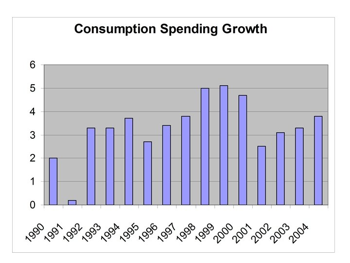
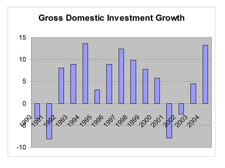
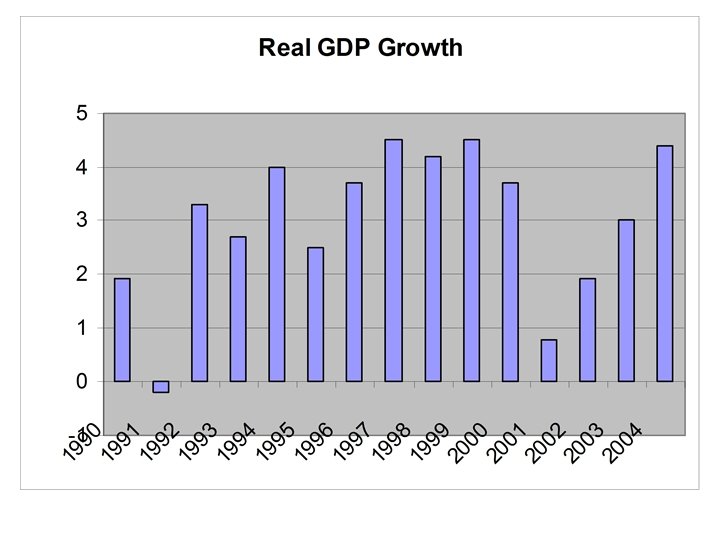
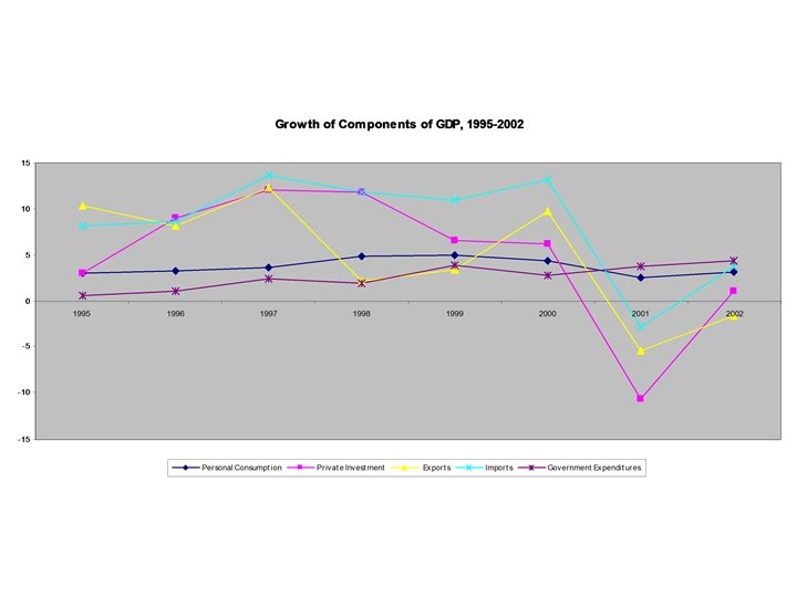
 Average Growth Rates by Component, 1996 -2000 8% 4
 Growth in components of Real GDP, 2000 -2003 Seasonally adjusted at annual rates
 Jobless Recovery Seasonally adjusted US unemployment rate Source: BEA
 Economy of Atlanta in the recession and jobless recovery Source: BLS
 A side-note: Job recovery in Atlanta
 Classical View • The Invisible Hand logic • Flexible Economy – – Dominated by small firms Recessionary pressure translates into deflation Price mechanism as a corrective tool Rapid price adjustments • Say’s Law: Supply Creates Its Own Demand
 Keynesian Points • Price flexibility is too strong of an assumption – Non-flexible input prices in the short-run leading to output adjustments • Decline in Expenditures Components of the GDP (Aggregate Demand) – The Thrift Paradox – Consumption spending and other factors • Under-Production as an equilibrium in the shortrun
 Income defined in terms of aggregate expenditures Y=C+I+G+X–M • Consumption") Aggregate Framework • (GPD) Income defined in terms of aggregate expenditures Y=C+I+G+X–M • Consumption Function C = a + mpc (Y – TAX) – Induced versus autonomous expenditure • Multiplier effect
Aggregate Framework • (GPD) Income defined in terms of aggregate expenditures Y=C+I+G+X–M • Consumption Function C = a + mpc (Y – TAX) – Induced versus autonomous expenditure • Multiplier effect
 Autonomous Expenditures 1. Independent of current income Autonomous Consumption 1. 2. Domestic Investment 1. 3. Is not a function of current income, but may be a function of future income, expected profitability, relative profitability, interest rate… Government Spending 1. 4. Consumption that does not depend on current income but depends on other factors (like future income, confidence, subsistence needs) Function of policy, and hence should not be considered as induced spending Exports 1. Exports tend to be a function of economic condition of the importing country. The wealthier it is, the more likely it is to purchase more Induced Expenditures • Function of current income Induced Consumption – Consumption that is driven by current income • Imports – note that imports do depend on the current income level. We will buy more of all goods, domestic or foreign in our incomes increase. Thus, it is an induced expenditure, but we will ignore this in our class and treat it as autonomous! There also other factors (other than income) that influence imports: relative prices, and hence the exchange rate, preferences…)
 More on the multiplier – simple example • Consider the following case – The level of private consumption spending is 500 million – The level of investment is 100 million – Current government spending is 100 million – Exports: 100 million; Imports: 50 million • Given this information we can conclude that the level of the GDP is 750 million. Now imagine that the government wants to increase that level to 800 million. What can the government do? – Natural conclusion is to increase the government spending by 50 million to close the gap between the actual and targeted GDP, but that actually is wrong. This ignores the multiplier effect. Assume that the MPC is 0. 8, in other words, 80% of the marginal dollar earned is directed into consumption, and hence becomes an income to someone else. In this case, using the math from our previous slides, the multiplier is 1/0. 2=5. Thus, an increase in government spending (autonomous expenditures component) will increase the GDP by 5 times the initial change through the multiplication effect. In this case, an increase in government spending of only 10 million to 110 million would suffice.
 More on the previous example • Now consider the example from the previous slide, but assume that the investment level declines by 5 million what will the implication to the GDP will be and what should the government do? – Note that investment is an autonomous component, and hence its decline will create a multiplication effect. The total decline will be 25 million, hence the GDP declines to 725 million – If the government selects to offset this change in investment spending through government spending, the change would have to be exactly equal to the drop in investment, i. e. 5 million. Note that although this policy will cure the recession caused by the investment decline, it will create another problem, the size of the government sector relative to the private sector has just increased…
 Further complication – note this slide will not appear on the exam • Now, let’s introduce income taxes…. • C = a + mpc (Y – t Y) – Here t represents the income tax rate, the rest of the function is the same • The new multiplier is: 1/(1 -mpc[1 -t]) – Note that income tax tends to reduce the multiplier effect as it increases the flow out of the consumption cycle. – Income taxes also present a second fiscal policy instrument: change in taxes • More complications can be introduced into the model, but as you can see their introduction does not complicate the math of the model
 Multiplier • Dollar spent on domestic consumption becomes an income of domestic workers/capital owners… • Marginal propensity to consume – fraction of the next dollar earned that will be directed into consumption • Multiplier = 1 / marginal leakage rate from the consumption stream
 Representing Aggregate Framework as Demand – Aggregate Demand • GDP expenditures as Aggregate Demand • Choice of axis variables: Output, Price Level • Nature of the slope of AD – – Wealth effect (real balances effect) Interest rate effect International substitution effect Multiplier effect
 Shifts in the AD Anything that changes autonomous expenditures shifts the AD • Consumer spending – Expectations about future (consumer confidence) • Investment – Interest rate (foreign rates) – Business confidence (stock market? ) • Exports/Imports – Exchange rate – Foreign economic conditions – International regulations…. • Government Spending – Fiscal policy
 Aggregate Supply • Long-Run – Classical view – Capacity level – Long-term Growth • Short-Run – Fixed input prices – Relationship between the price level and the output: CPI and Q
 equilibrium • Long-Run and Short-Run • Demand Driven Recession – Deflationary pressure – Long-run input cost adjustment – Possible need for government intervention in the short -run • Supply Driven Recession – Input cost rise – Inflationary pressure • Eliminating Recession through Demand Side Policy
 Fiscal Stabilization Policy • Instruments – Government Spending – Taxes – Transfers – Budget • Ability to be targeted – State level – Municipality level
 Drawbacks of Fiscal Expansion note that this is in chapter 30 • crowding-out effects [these refer to the replacement of one sector by another, in the case of expansionary fiscal policy, the public sector displaces the private sector] – direct [direct provision. GSU reduces the demand for Emory] – indirect [this works through the interest rate mechanism, expansionary fiscal policy results in government borrowing, the current tax cut and budget deficit is a perfect example of that, government borrowing may lead to an increase in the interest rates and hence higher costs for private sector investment] – open-economy effect [an increase in the interest rate due to government borrowing may cause an influx of foreign investment and therefore drive up the value of domestic currency] – Time lags (decision, recognition, effect) Ideally the second exam will be here
 Monetary Side MONEY • Functions of money – Medium of exchange – Unit of account – Store of value • Measuring the supply of money (liquidity and transaction principles) – M 1 • Cash, checking accounts, traveler’s checks – M 2 • M 1+savings accounts, CD accounts, money market accounts
 Money Creation by Banks • Creation of money balances by banks – Fractional reserve system and lending – Money multiplier • Potential • Actual • Regulatory institutions – Federal Reserve Bank – FDIC
 • Goal of") Monetary Policy • Federal Reserve Bank of the US (Central Bank) • Goal of the Policy – Influence consumption and investment spending – Change the exchange rate side effect more than a goal • Policy Instruments – Open Market Operations – Discount Rate – Reserve Requirements • Policy Operating Targets – Federal Funds Rate • Weaknesses of the Policy – Liquidity trap – Recognition/time lags
Monetary Policy • Federal Reserve Bank of the US (Central Bank) • Goal of the Policy – Influence consumption and investment spending – Change the exchange rate side effect more than a goal • Policy Instruments – Open Market Operations – Discount Rate – Reserve Requirements • Policy Operating Targets – Federal Funds Rate • Weaknesses of the Policy – Liquidity trap – Recognition/time lags
 Does Dollar Matter?
 Should We Be Concerned With The Fluctuating Dollar? • TRADE and Currency Fluctuations – Price Changes – Standard of Living – Commodity Prices Date USD per EURO USD Price of OIL Euro Price of OIL March 1, 2002 0. 8652 22. 40 25. 89 March 3, 2003 1. 0835 35. 88 33. 11 March 1, 2004 1. 2431 36. 86 29. 65 March 1, 2005 1. 3189 51. 68 39. 18 % change over the period 52. 44 130. 71 51. 35
 The For. Ex market • Supply of the USD – Imports to the US • Goods (trade) • Services (tourism) – US investment abroad • Foreign Financial Markets • Direct investment abroad – Central Banks – Speculation • Demand for the USD – US Exports • Goods • Services (tourism) – Foreign Investment into US • US Financial markets • Direct investment – Central Banks – Speculation
 The Interesting 90’s • 1991 -92: Collapse of the USSR Block, beginning of the Transitional Recession in Eastern Europe • 1994 Mexican Currency Crisis • 1991(2)-95 The Balkan Wars • 1998 Recession in Japan • 1997 (July) Beginning of the Asian Financial Crisis • 1998 major Rouble Crisis US ECONOMY average % rates 19922000 20012004 Real GDP 3. 7 2. 5 Gross Domestic Private Investment 8. 7 1. 8 Non-Residential Investment 9. 1 0. 2
 The market for USD in the 90’s P of USD Influx of investment stimulated Demand D S Increase in imports stimulated Supply Demand Effect Dominated (thus positively effecting consumers’ standard of living)
 The post 90’s era • United Europe – 10 New Countries Entered the Union on May 1 st of 2004, bringing the total number of member states to 25, with combined population of over 430 million (US population is 293 million). • • • Strong Growth in Russia and China Emerging Economies of Brazil and India Threat of Terrorism to the US Continuous Growth in US Trade Deficit More Recently, the French and Dutch Referendums on the EU Constitution
 The BIG picture • • Rise in Imports Increase in Supply Depreciation Rise in Exports Increase in Demand Appreciation Influx of Investment Increase in Demand Appreciation Outflow of Investment Increase in Supply Depreciation • BALANCE OF PAYMENTS – An Economy’s International Balance Sheet (www. bea. gov)
 Balance of Payments • Current Account – Trade – Income flow • Financial Account – Investment Flow • Paying for Foreign Goods with Domestic Financial Assets – the US Example (US Bo. P)
 Floating Exchange Rate Regime – Currency") Currency Trade and Exchange Regime (History – optional) Floating Exchange Rate Regime – Currency Trade by Central Banks – (Forward looking instruments – optional) Fixed Exchange Rate Regime – Does Recent Dollar Depreciation Impact the Trade Deficit with CHINA? – Price Stabilization and Fixed Exchange Rate Regime – Risk to CB
Currency Trade and Exchange Regime (History – optional) Floating Exchange Rate Regime – Currency Trade by Central Banks – (Forward looking instruments – optional) Fixed Exchange Rate Regime – Does Recent Dollar Depreciation Impact the Trade Deficit with CHINA? – Price Stabilization and Fixed Exchange Rate Regime – Risk to CB