Economic Simulations Using Mathematica Kota Minegishi Outline

Economic Simulations Using Mathematica Kota Minegishi

Outline 1. 2. 3. 4. Objectives Notional Demand Driven Economies Effective Demand Driven Economies Conclusions

1. Objectives Q. Why economic simulations? A. Economic simulations allow us to § § Understand existing theories better Change some assumptions in theories Light existing theories from different angles Improve our intuitions on economic theories

1. Objectives Our Targets ü Setup and compare models for: Notional Demand Driven Economies § The Walrasian Auctioneer Effective Demand Driven Economies § Triangular Trade ü To Show Simulations in Mathematica § Iterations § Modified assumptions in theories § Graphical interpretations

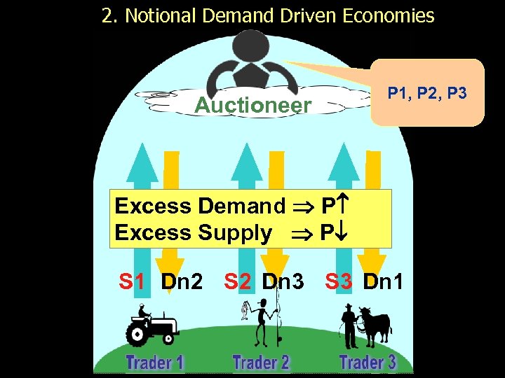2. Notional Demand Driven Economies Auctioneer P 1, P 2, P 3 Excess Demand P Excess Supply P S 1 Dn 2 S 2 Dn 3 S 3 Dn 1

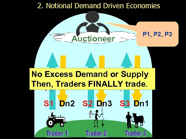2. Notional Demand Driven Economies Auctioneer P 1, P 2, P 3 No Excess Demand or Supply Then, Traders FINALLY trade. S 1 Dn 2 S 2 Dn 3 S 3 Dn 1

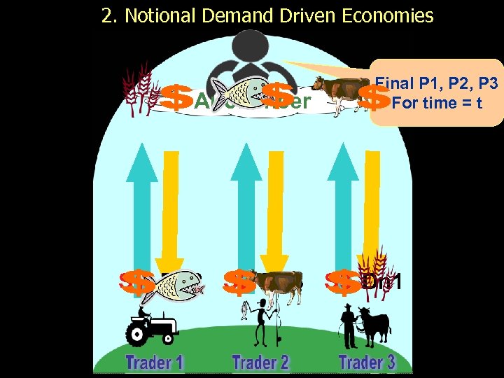2. Notional Demand Driven Economies Auctioneer Final P 1, P 2, P 3 For time = t S 1 Dn 2 S 2 Dn 3 S 3 Dn 1

2. Notional Demand Driven Economies Ideas For Implementation § Define traders’ supply functions § Define traders’ utility functions and budget constraints derive demand functions § Solve di = si for i = 1, 2, 3 simultaneously for {p 1, p 2, p 3} § With these price equations, define equations for quantities, money holding, and GDP over time.

Utility Maximizing Behavior 3 D 2 D From [1], [2], & [3], obtain local extrema (x, y) and Lagrange multiplier λ

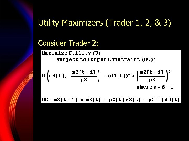Utility Maximizers (Trader 1, 2, & 3) Consider Trader 2;

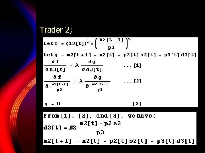Trader 2;

2. Notional Demand Driven Economies Definitions A 1; si[t] = di[t] m 1[t] = m 1[t - 1] + p 1[t] s 1[t] - p 2[t] d 2[t] m 2[t] = m 2[t - 1] + p 2[t] s 2[t] - p 3[t] d 3[t] m 3[t] = m 3[t - 1] + p 3[t] s 3[t] - p 1[t] d 1[t] = β 2 (m 3[t] + p 3[t] s 3[t]) / p 1[t] d 3[t] = β 1 (m 2[t] + p 2[t] s 2[t]) / p 3[t] d 2[t] = β 3 (m 1[t]+ p 1 [t] s 1[t]) / p 2[t] s 1[t] = γ 1 p 1[t] s 2[t] = γ 2 p 2[t] s 3[t] = γ 3 p 3[t]

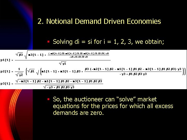2. Notional Demand Driven Economies § Solving di = si for i = 1, 2, 3, we obtain; § So, the auctioneer can “solve” market equations for the prices for which all excess demands are zero.

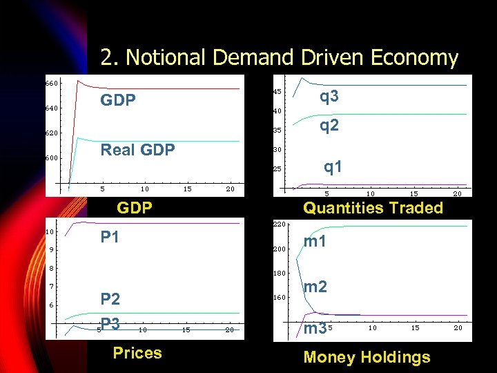2. Notional Demand Driven Economy GDP q 3 q 2 Real GDP P 1 P 2 P 3 Prices q 1 Quantities Traded m 1 m 2 m 3 Money Holdings

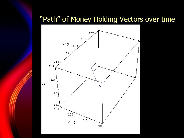“Path” of Money Holding Vectors over time

2. Notional Demand Driven Economies § As time [t] elapses, the economy will find the general equilibrium * under well known conditions such as; § § § the weak axiom of revealed preferences gross substitutions a dominant diagonal § At the general equilibrium, all variables stop changing over time [t]. *Roberts and Schultz, Modern Mathematical and Economic Analysis, pp 304.

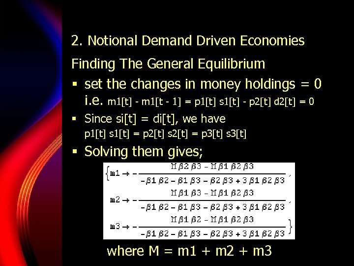2. Notional Demand Driven Economies Finding The General Equilibrium § set the changes in money holdings = 0 i. e. m 1[t] - m 1[t - 1] = p 1[t] s 1[t] - p 2[t] d 2[t] = 0 § Since si[t] = di[t], we have p 1[t] s 1[t] = p 2[t] s 2[t] = p 3[t] s 3[t] § Solving them gives; where M = m 1 + m 2 + m 3

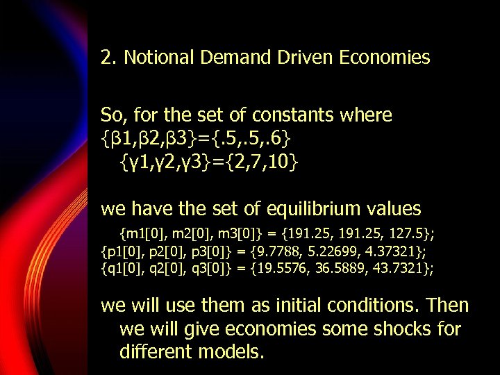2. Notional Demand Driven Economies So, for the set of constants where {β 1, β 2, β 3}={. 5, . 6} {γ 1, γ 2, γ 3}={2, 7, 10} we have the set of equilibrium values {m 1[0], m 2[0], m 3[0]} = {191. 25, 127. 5}; {p 1[0], p 2[0], p 3[0]} = {9. 7788, 5. 22699, 4. 37321}; {q 1[0], q 2[0], q 3[0]} = {19. 5576, 36. 5889, 43. 7321}; we will use them as initial conditions. Then we will give economies some shocks for different models.

Vector field of {m 1’[t], m 2’[t], m 3’[t] } {β 1, β 2, β 3}= {. 5, . 6} The long run equilibrium

Vector field of {m 1’[t], m 2’[t], m 3’[t] } {β 1, β 2, β 3}= {. 5, . 6} The long run equilibrium

Vector field of {m 1’[t], m 2’[t], m 3’[t] } {β 1, β 2, β 3}= {. 5, . 6} The long run equilibrium

2. Notional Demand Driven Economies Q. Why do prices adjust even when demands are notional? A. There is the auctioneer in this economy. Agents trade with the auctioneer.

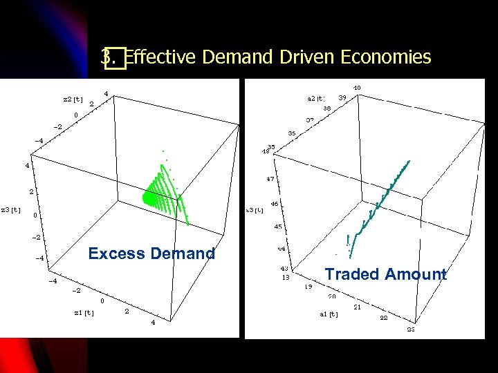
3. Effective Demand Driven Economies § Notional Demands § Budget Constraints § Effective Demands § Budget Constraints and Other Constraints § e. g. If a trader could not sell, then he cannot buy as much as he wanted.

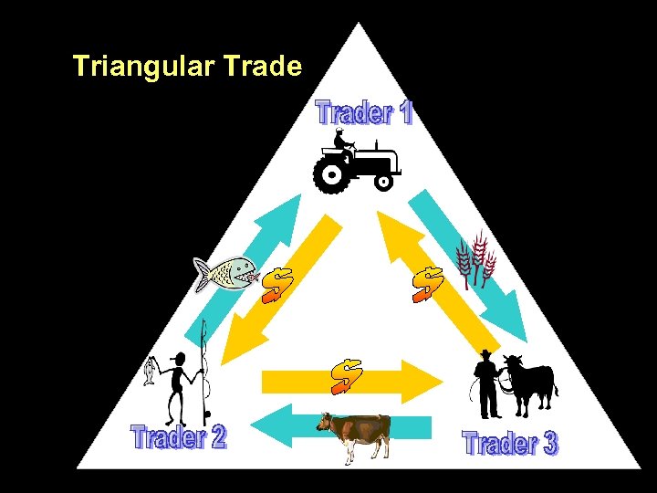Triangular Trade

3. Effective Demand Driven Economies Ideas For Implementation § Have Trader 1 be an initiator of trades and Trader 2 be utility maximizers § Create variables for actual traded quantities ( ai= min[ di, si ] ) so that traders will adjusting budget constrains according to them

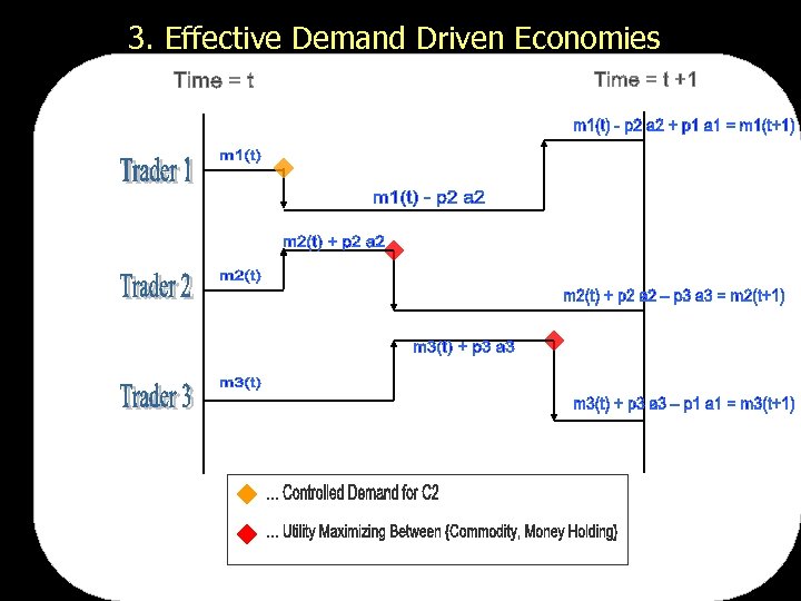3. Effective Demand Driven Economies

3. Effective Demand Driven Economies Definitions B 1; ai[t] actual traded q’s m 1[t] = m 1[t - 1] + p 1[t-1] a 1[t - 1] - p 2[t-1] a 2[t - 1] m 2[t] = m 2[t - 1] + p 2[t-1] a 2[t - 1] - p 3[t-1] a 3[t - 1] m 3[t] = m 3[t - 1] + p 3[t-1] a 3[t - 1] - p 1[t-1] a 1[t - 1] d 1[t] = β 2 (m 3[t] + p 3[t] a 3[t]) / p 1[t] d 3[t] = β 1 (m 2[t] + p 2[t] a 2[t]) / p 3[t] d 2[t] = β 3 (m 1[t]+ p 1[t] s 1[t])a 1[t]=min[s 1[t], /p 2[t] s 1[t] = γ 1 p 1[t] s 2[t] = γ 2 p 2[t] s 3[t] = γ 3 p 3[t] d 1[t] a 2[t]=min[s 2[t], d 2[t]] a 3[t]=min[s 3[t], d 3[t]]]

3. Effective Demand Driven Economies Definitions B 2; price adjustments z 1[t] = d 1[t] - s 1[t] z 2[t] = d 2[t] - s 2[t] z 3[t] = d 3[t] - s 3[t] p 1[t] = p 1[t - 1] + k 1*z 1[t - 1] p 2[t] = p 2[t - 1] + k 2*z 2[t - 1] p 3[t] = p 3[t - 1] + k 3*z 3[t - 1]

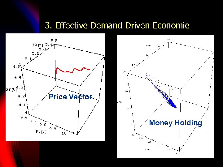
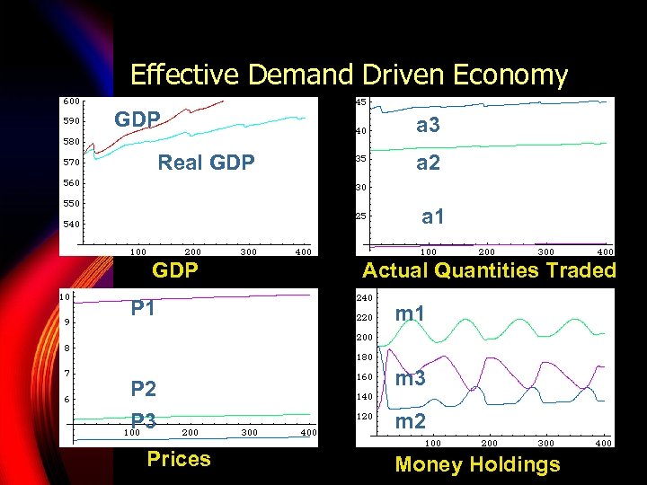Effective Demand Driven Economy GDP Real GDP a 3 a 2 a 1 GDP Actual Quantities Traded P 1 m 1 P 2 m 3 P 3 m 2 Prices Money Holdings

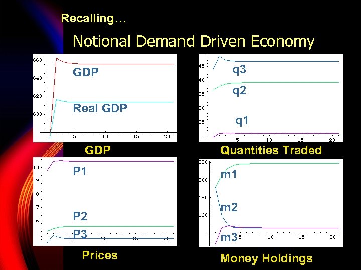Recalling… Notional Demand Driven Economy GDP q 3 q 2 Real GDP P 1 P 2 P 3 Prices q 1 Quantities Traded m 1 m 2 m 3 Money Holdings

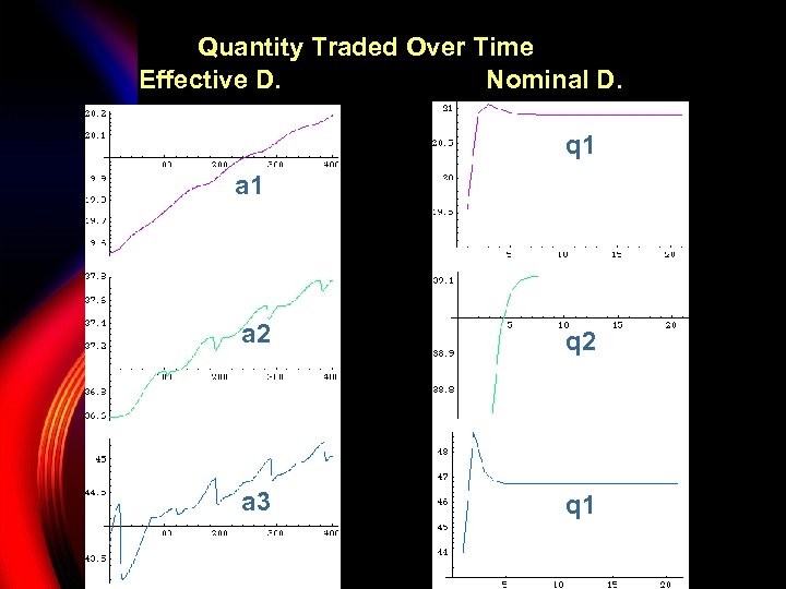Quantity Traded Over Time Effective D. Nominal D. q 1 a 2 q 2 a 3 q 1

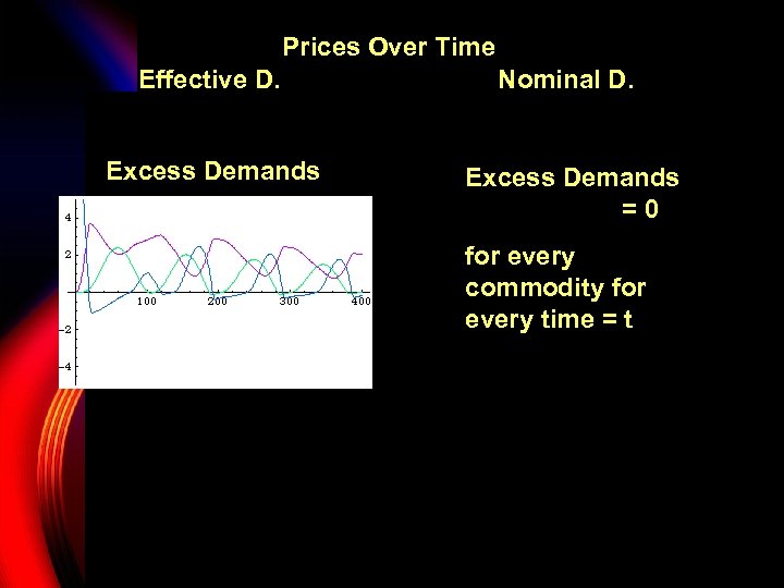Prices Over Time Effective D. Nominal D. Excess Demands P 1 Excess Demands =0 for every commodity for P 2 every time = t P 2 P 3

3. Effective Demand Driven Economies Excess Demand Traded Amount

3. Effective Demand Driven Economie Price Vector Money Holding

Comparison of GDP[t] Paths over time Notional. D Effective. D 2: 0. 5 0. 6 Trader 2 prefers to buy more and hold less

Comparison of GDP[t] Paths over time Notional. D Half-Notional. D Effective. D 2: 0. 5 0. 6 Trader 2 prefers to buy more and hold less

Comparison of GDP[t] Paths over time Notional. D Half-Notional. D Effective. D. Supplies Fixed 2: 0. 5 0. 6 Trader 2 prefers to buy more and hold less

Comparison of GDP[t] Paths over time Notional. D Trader 1 expects his sales *P, S-fixed Trader 1 buys a fixed amount 2: 0. 5 0. 6 Trader 2 prefers to buy more and hold less

Comparison of GDP[t] Paths over time Notional. D Effective. D Initial conditions: For the first two periods, Trader 2 decided to buy less.

4. Conclusions We have shown; The difference b/w Notional and Effective demands § the Walrasian Auctioneer § Triangular Trade Economic simulations § § Improve Our Understanding of the Neoclassical theory Have modified assumptions Light theory from different angles Improve our intuitions on economic theories Economic Simulations using Mathematica § iterations § modified assumptions § graphical interpretations

Any Questions?