Economic Policies and Efficiency Exercises and Applications Lecture

Economic Policies and Efficiency: Exercises and Applications Lecture 6 – academic year 2013/14 Introduction to Economics Fabio Landini

Ex. 6. 2 – Tax on petrol (I) Question The European Parliament decides that the EU must decrease the level of air pollution by reducing the use of petrol in road transports. Therefore, it introduces a tax on petrol of 0. 50 € a litre. Should the EU introduce a tax on consumption or production? Explain in detail by using a graphical representation (S&D model). 2

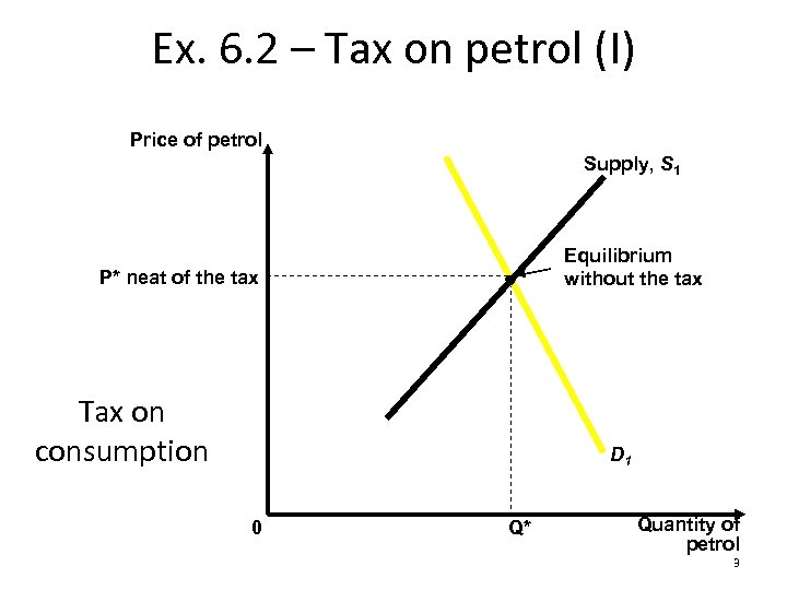Ex. 6. 2 – Tax on petrol (I) Price of petrol Supply, S 1 Equilibrium without the tax P* neat of the tax Tax on consumption D 1 0 Q* Quantity of petrol 3

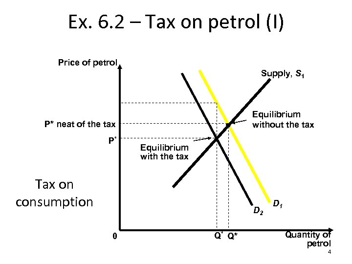Ex. 6. 2 – Tax on petrol (I) Price of petrol Supply, S 1 Equilibrium without the tax P* neat of the tax P* Equilibrium with the tax Tax on consumption D 2 0 Q* Q* D 1 Quantity of petrol 4

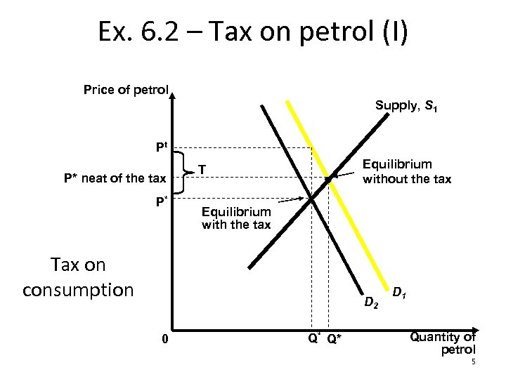Ex. 6. 2 – Tax on petrol (I) Price of petrol Supply, S 1 Pt P* neat of the tax P* Equilibrium without the tax T Equilibrium with the tax Tax on consumption D 2 0 Q* Q* D 1 Quantity of petrol 5

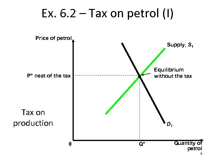Ex. 6. 2 – Tax on petrol (I) Price of petrol Supply, S 1 Equilibrium without the tax P* neat of the tax Tax on production D 1 0 Q* Quantity of petrol 6

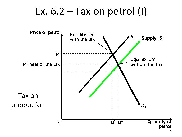Ex. 6. 2 – Tax on petrol (I) Price of petrol Equilibrium with the tax S 2 P* Supply, S 1 Equilibrium without the tax P* neat of the tax Tax on production D 1 0 Q* Q* Quantity of petrol 7

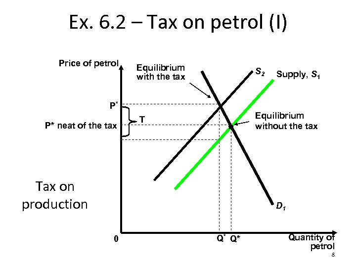Ex. 6. 2 – Tax on petrol (I) Price of petrol Equilibrium with the tax S 2 P* P* neat of the tax Supply, S 1 Equilibrium without the tax T Tax on production D 1 0 Q* Q* Quantity of petrol 8

Ex. 6. 2 – Tax on petrol (I) Taxes on consumption or production generates the same effects on the market A positive difference is created between the price paid by the consumer and the one paid by the producer This difference is indeed the same, independently on whether the tax is imposed on production or consumption 9

Ex. 6. 2 – Tax on petrol (II) Question If the demand for petrol were more elastic, would this tax be more or less efficient in reducing the quantity of petrol that is consumed? Explain in detail by using a graphical representation (S&D model). 10

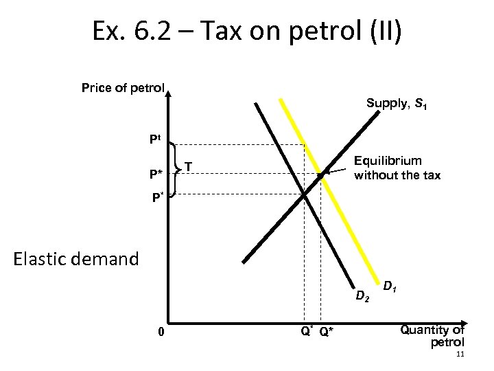Ex. 6. 2 – Tax on petrol (II) Price of petrol Supply, S 1 Pt P* Equilibrium without the tax T P* Elastic demand D 2 0 Q* Q* D 1 Quantity of petrol 11

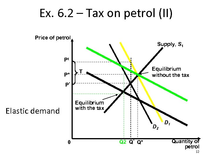Ex. 6. 2 – Tax on petrol (II) Price of petrol Supply, S 1 Pt P* Equilibrium without the tax T P* Equilibrium with the tax Elastic demand D 2 0 Q 2 Q* Q* D 1 Quantity of petrol 12

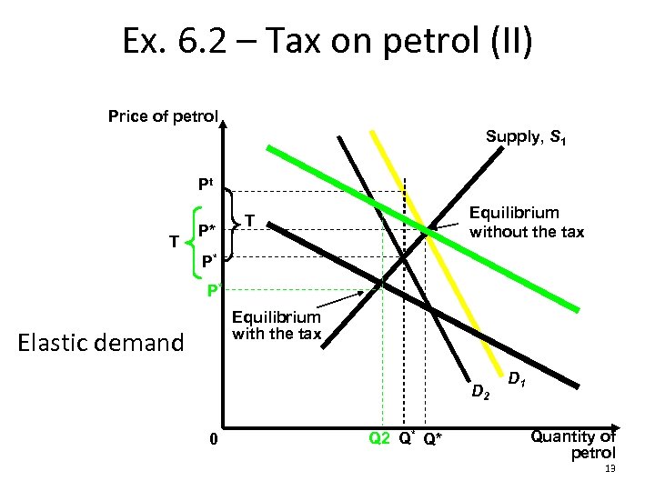Ex. 6. 2 – Tax on petrol (II) Price of petrol Supply, S 1 Pt T P* Equilibrium without the tax T P* P* Equilibrium with the tax Elastic demand D 2 0 Q 2 Q* Q* D 1 Quantity of petrol 13

Ex. 6. 2 – Tax on petrol (II) With a higher elasticity ED(p), the same tax would induce a greater reduction in the equilibrium quantity 14

Ex. 6. 2 – Tax on petrol (III) Question Do the consumers of petrol obtain some benefits from the introduction of of the tax? Do the workers of the petrol industry obtain some benefits from the introduction of the tax? 15

Ex. 6. 2 – Tax on petrol (III) Answer Consumers suffer a cost from the introduction of the tax, because the latter has anyway a negative effect by increasing the market price. Workers of the petrol industry suffer a cost too, by reducing the quantity produced (in addition to the cost as consumers) 16

Ex. 6. 3 – Tax and prices Question Two market equations: QS = 2 P QD = 12 – P a) Find the equilibrium price and quantity; b) What happen if the Government imposes a tax T on producers? 17

Ex. 6. 3 – Tax and prices Answer a) Equilibrium price and quantity: QS = QD 2 P = 12 – P -> 3 P = 12 -> P = 4 and QO = QD = 8 18

Ex. 6. 3 – Tax and prices Answer b) Equilibrium after the tax T, steps: 1. Find equilibrium with the new supply curve 2. Compute the price paid by consumer 3. Compute the received by the producers 4. Compute the new quantity sold in equilibrium 19

Ex. 6. 3 – Tax and prices If a tax T is introduced the price paid by the consumers is: QS = QD 2(P-T) = 12 – P 2 P - 2 T = 12 – P 3·P = 12 + 2·T P = 4 + 2/3·T 20

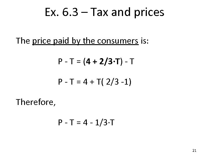Ex. 6. 3 – Tax and prices The price paid by the consumers is: P - T = (4 + 2/3·T) - T P - T = 4 + T( 2/3 -1) Therefore, P - T = 4 - 1/3·T 21

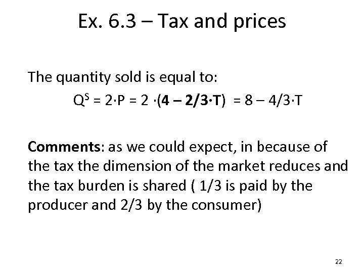Ex. 6. 3 – Tax and prices The quantity sold is equal to: QS = 2·P = 2 ·(4 – 2/3·T) = 8 – 4/3·T Comments: as we could expect, in because of the tax the dimension of the market reduces and the tax burden is shared ( 1/3 is paid by the producer and 2/3 by the consumer) 22

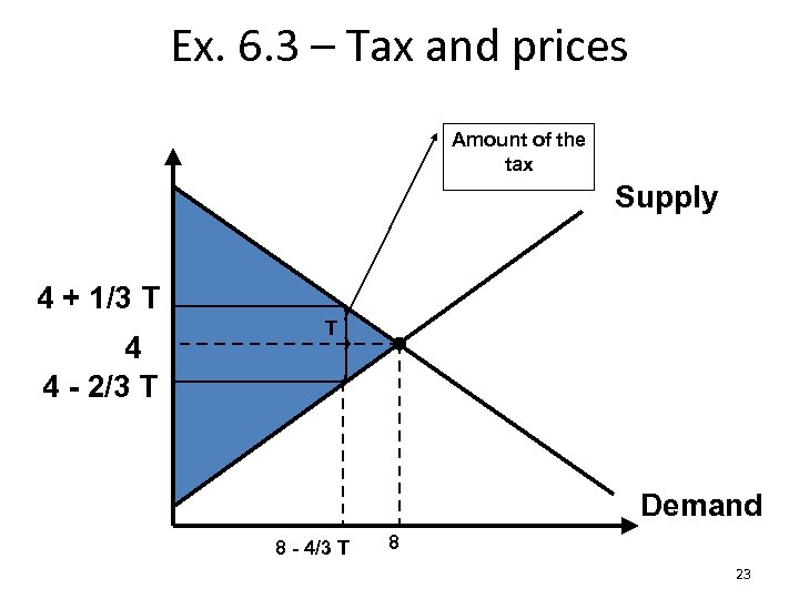Ex. 6. 3 – Tax and prices Amount of the tax Supply 4 + 1/3 T 4 4 - 2/3 T T Demand 8 - 4/3 T 8 23

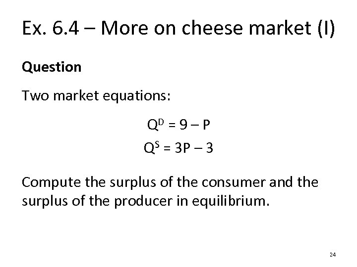Ex. 6. 4 – More on cheese market (I) Question Two market equations: QD = 9 – P QS = 3 P – 3 Compute the surplus of the consumer and the surplus of the producer in equilibrium. 24

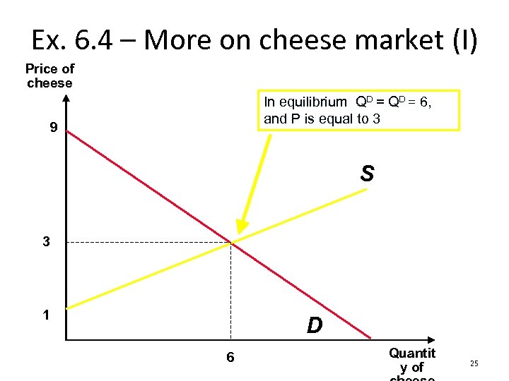Ex. 6. 4 – More on cheese market (I) Price of cheese In equilibrium QD = 6, and P is equal to 3 9 S 3 1 D 6 Quantit y of 25

Ex. 6. 4 – More on cheese market (I) To compute the surplus of consumer (RC) we must compute the size of the area between the demand curve and the equilibrium price. To compute the surplus of producer (RP) we must compute the size of the are between the supply curve and the equilibrium price. 26

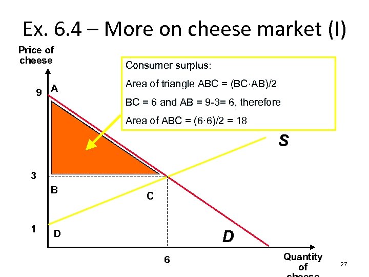Ex. 6. 4 – More on cheese market (I) Price of cheese 9 A Consumer surplus: Area of triangle ABC = (BC·AB)/2 BC = 6 and AB = 9 -3= 6, therefore Area of ABC = (6· 6)/2 = 18 S 3 B 1 C D D 6 Quantity of 27

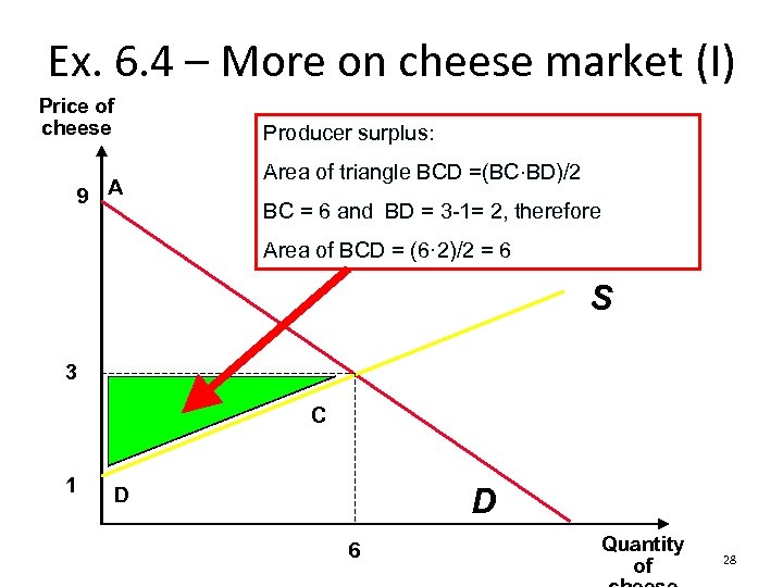Ex. 6. 4 – More on cheese market (I) Price of cheese 9 A Producer surplus: Area of triangle BCD =(BC·BD)/2 BC = 6 and BD = 3 -1= 2, therefore Area of BCD = (6· 2)/2 = 6 S 3 B 1 C D D 6 Quantity of 28

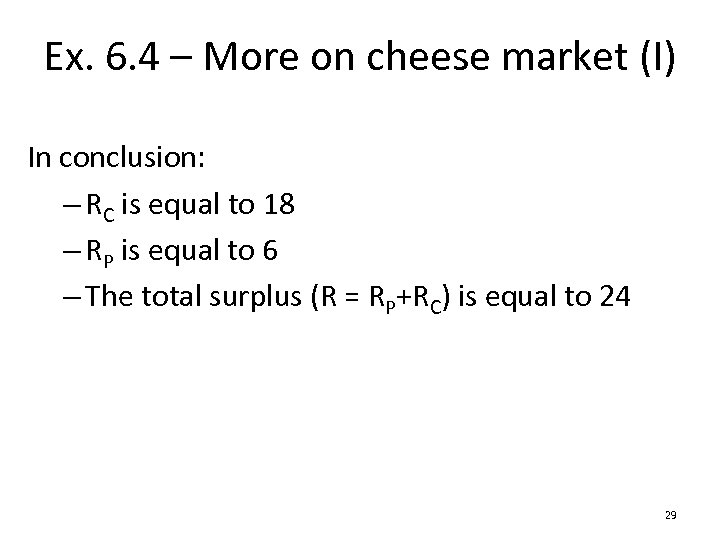Ex. 6. 4 – More on cheese market (I) In conclusion: – RC is equal to 18 – RP is equal to 6 – The total surplus (R = RP+RC) is equal to 24 29

Ex. 6. 4 – More on cheese market (II) Question The government decides that the price of cheese that is determined on the market is too low. Suppose that the Government introduces a minimum price. Draw the S&D graph and show the effect of such policy on the market price and on the quantity sold. Does this intervention induce scarcity or excess supply? 30

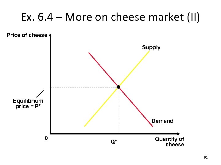Ex. 6. 4 – More on cheese market (II) Price of cheese Supply Equilibrium price = P* Demand 0 Q* Quantity of cheese 31

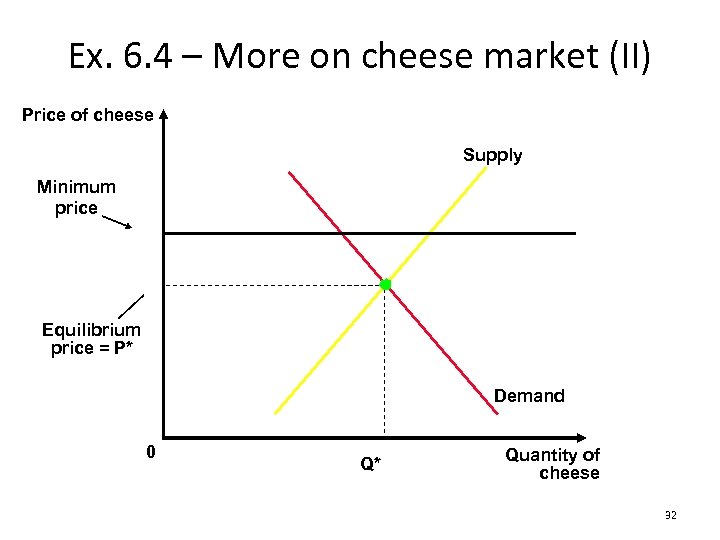Ex. 6. 4 – More on cheese market (II) Price of cheese Supply Minimum price Equilibrium price = P* Demand 0 Q* Quantity of cheese 32

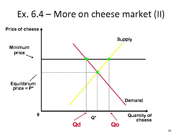Ex. 6. 4 – More on cheese market (II) Price of cheese Supply Minimum price Equilibrium price = P* Demand 0 Q* Qd Qo Quantity of cheese 33

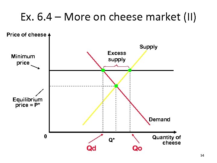Ex. 6. 4 – More on cheese market (II) Price of cheese Supply Excess supply Minimum price Equilibrium price = P* Demand 0 Q* Qd Qo Quantity of cheese 34

Ex. 6. 5 – More on cheese market (III) Question The farmers of a given country complains that the imposition of the minimum level of price on cheese has reduced their total revenue. Is it possible? Explain why. 35

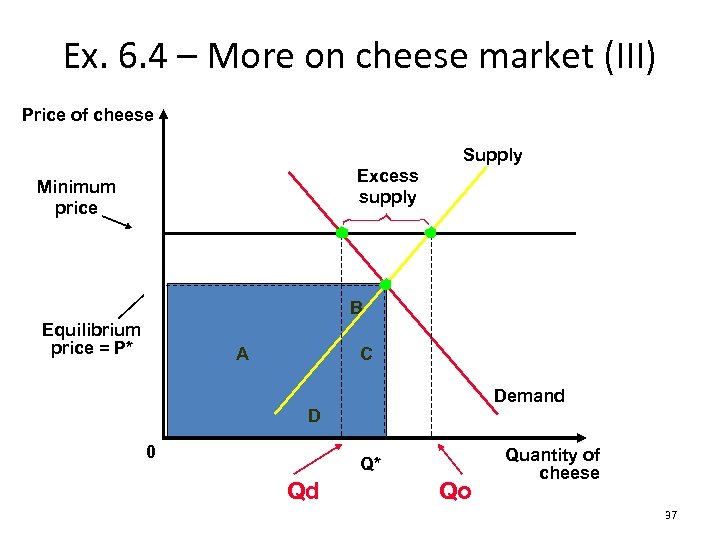
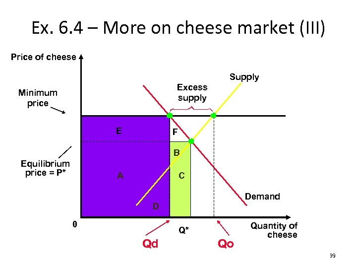
Ex. 6. 4 – More on cheese market (III) Answer The sign of the reduction in total revenue for farmer depends on the elasticity of demand with respect to price The total revenue before the introduction of the minimum level of prise is equal to (A+B+C+D) (next slide) 36

Ex. 6. 4 – More on cheese market (III) Price of cheese Supply Excess supply Minimum price B Equilibrium price = P* A C Demand D 0 Q* Qd Qo Quantity of cheese 37

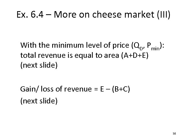Ex. 6. 4 – More on cheese market (III) With the minimum level of price (QD, Pmin): total revenue is equal to area (A+D+E) (next slide) Gain/ loss of revenue = E – (B+C) (next slide) 38

Ex. 6. 4 – More on cheese market (III) Price of cheese Supply Excess supply Minimum price E F B Equilibrium price = P* A C Demand D 0 Q* Qd Qo Quantity of cheese 39

Ex. 6. 4 – More on cheese market (IV) Question In response to the farmers’ complaints, the Government to buy all the excess supply of cheese from farmer at the limit price. In comparison with the introduction of the minimum price, a) Who benefits from this new intervention? b) Who is damaged? 40

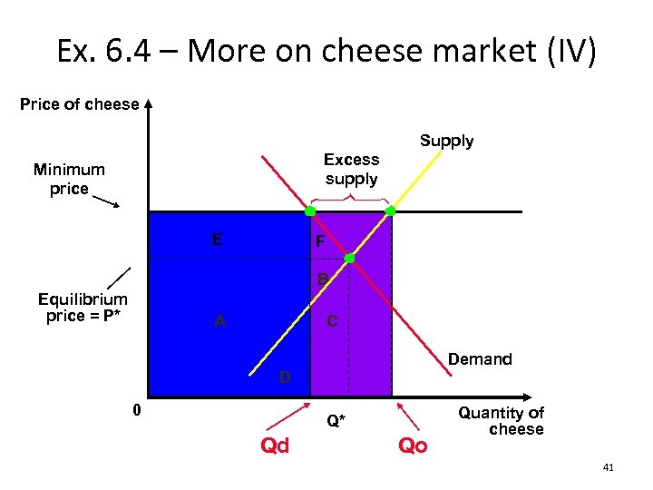Ex. 6. 4 – More on cheese market (IV) Price of cheese Supply Excess supply Minimum price E F B Equilibrium price = P* A C Demand D 0 Q* Qd Qo Quantity of cheese 41

Ex. 6. 4 – More on cheese market (IV) Answer The new intervention benefits farmers and damages taxpayers (if we assume that the Government finance the new policy by increasing taxes). 42

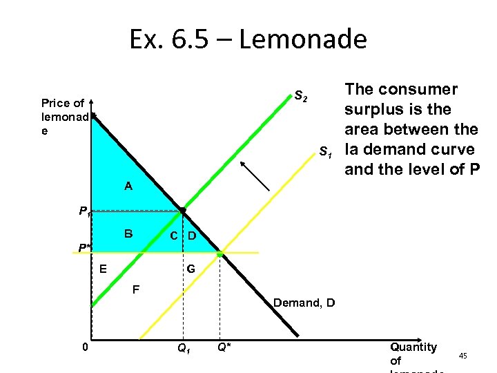
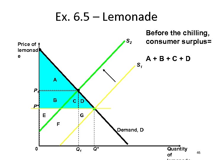
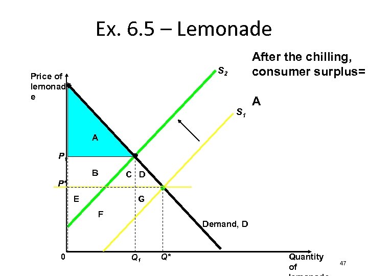
Ex. 6. 5 – Lemonade Question The (usual) chilling destroys part of the lemon harvest in Sicily. a) Which is the effect on the consumer surplus in the market for lemonade? b) What happen to the surplus of the lemonade producers? 43

Ex. 6. 5 – Lemonade Answer a) In the market for lemonade lemons are inputs –> the lemonade supply curve shifts leftward 44

Ex. 6. 5 – Lemonade S 2 Price of lemonad e S 1 The consumer surplus is the area between the la demand curve and the level of P A P 1 B P* E C D G F Demand, D 0 Q 1 Q* Quantity of 45

Ex. 6. 5 – Lemonade Before the chilling, consumer surplus= S 2 Price of lemonad e S 1 A+B+C+D A P 1 B P* E C D G F Demand, D 0 Q 1 Q* Quantity of 46

Ex. 6. 5 – Lemonade After the chilling, consumer surplus= S 2 Price of lemonad e S 1 A A P 1 B P* E C D G F Demand, D 0 Q 1 Q* Quantity of 47

Ex. 6. 5 – Lemonade Answer b) Effects on the lemonade producers surplus 48

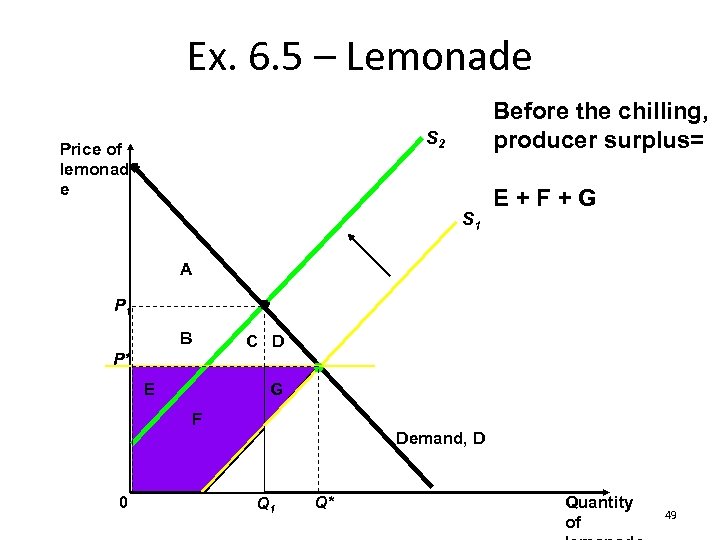Ex. 6. 5 – Lemonade Before the chilling, producer surplus= S 2 Price of lemonad e S 1 E+F+G A P 1 B P* E C D G F Demand, D 0 Q 1 Q* Quantity of 49

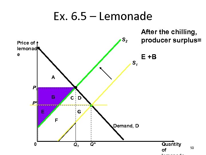Ex. 6. 5 – Lemonade After the chilling, producer surplus= S 2 Price of lemonad e S 1 E +B A P 1 B P* E C D G F Demand, D 0 Q 1 Q* Quantity of 50

Ex. 6. 5 – Lemonade Therefore: the effect on the consumer surplus in UNCERTAIN. It depends on the price elasticity of the demand curve. If the curve is flat (high elasticity), it is more likely that the producer will loose (area B gets smaller) 51