Econometrics Econ 405 Chapter 9 MULTICOLLINEARITY WHAT HAPPENS

Econometrics Econ. 405 Chapter 9: MULTICOLLINEARITY: WHAT HAPPENS IF THE REGRESSORS ARE CORRELATED

I. The Natural of Multicollinearity § Multicollinearity arises when a linear relationship exists between two or more independent variables in a regression model. § It practice, you rarely encounter perfect multicollinearity, but high multicollinearity is quite common. § There are two types of multicollinearity.

1 - Perfect multicollinearity: § Occurs when two or more independent variables in a regression model exhibit a deterministic ( perfectly predictable) linear relationship. § Perfect multicollinearity violates one of the CLRM assumptions. § In such a case, OLS can not be used to estimate the value of parameters (β’s).

2 - High multicollinearity: § it results from a linear relationship between your independent variables with a high degree of correlation but aren’t completely deterministic. § It is much more common than its perfect counterpart and can be equally problematic when it comes to estimating an econometric model. § In practice, when econometricians point to a multicollinearity issue, they are typically referring to high multicollinearity rather than perfect multicollinearity.

§ Technically, the presence of high multicollinearity does not violate any CLRM assumption. § Consequently, OLS estimates can be obtained and are BLUE with high multicollinearity.

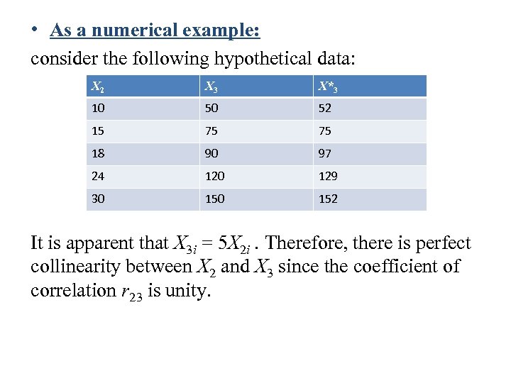• As a numerical example: consider the following hypothetical data: X 2 X 3 X*3 10 50 52 15 75 75 18 90 97 24 120 129 30 152 It is apparent that X 3 i = 5 X 2 i. Therefore, there is perfect collinearity between X 2 and X 3 since the coefficient of correlation r 23 is unity.

• The variable X*3 was created from X 3 by simply adding to it the following numbers, which were taken from a table of random numbers: 2, 0, 7, 9, 2. • Now there is no longer perfect collinearity between X 2 and X*3 as of (X 3 i = 5 X 2 i + vi ). However, the two variables are highly correlated because calculations will show that the coefficient of correlation between them is 0. 9959.

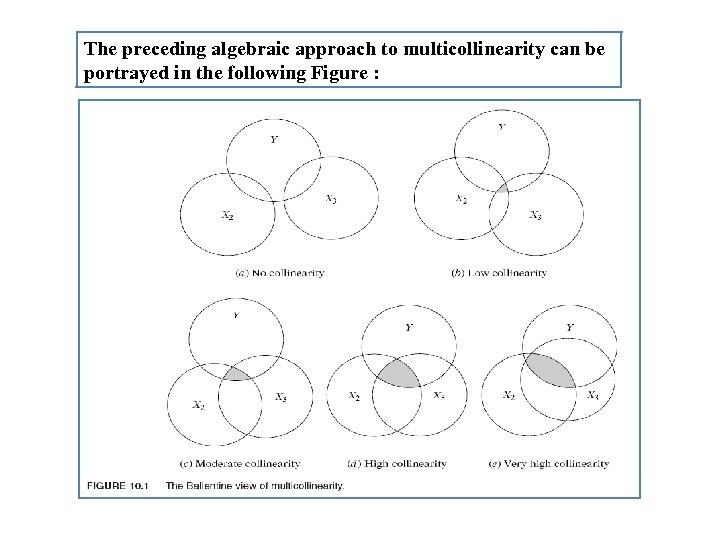The preceding algebraic approach to multicollinearity can be portrayed in the following Figure :

II. Sources of Multicollinearity There are several sources of multicollinearity; 1. The data collection method employed: for example, sampling over a limited range of the values taken by the regressors in the population. 2. Constraints on the model or in the population being sampled: For example, in the regression of electricity consumption (Y) on income (X 2) and house size (X 3) (High X 2 always mean high X 3).

3. Model specification: for example, adding polynomial terms to a regression model, especially when the range of the X variable is small. 4. An overdetermined model: This happens when the model has more explanatory variables than the number of observations. 5. Common time trend component: especially in time series data, may be that the regressors included in the model share a common trend, that is, they all increase or decrease over time.

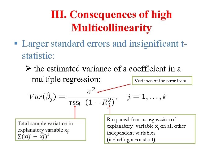III. Consequences of high Multicollinearity § Larger standard errors and insignificant tstatistic: Ø the estimated variance of a coefficient in a multiple regression: Variance of the error term R-squared from a regression of explanatory variable xj on all other independent variables (including a constant)

•

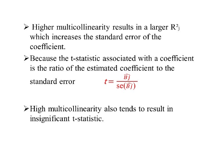§ Coefficient estimates that are sensitive to changes in specification: Ø If the IVs are highly collinear, the estimates must emphasize small differences in the variables in order to assign an independent effect to each of them. ØAdding or removing variables from the model can change the nature of the small differences and drastically change your coefficient estimates. In other words, your result s aren’t robust.

§ Nonsensical coefficient signs and magnitudes: Ø with higher multicollinearity, the variance of the estimated coefficients increases, which in turn increases the changes of obtaining coefficient estimates with extreme values. ØConsequently, these estimates my have unbelievably large magnitudes and/or signs that counter the expected relationship between IVs and DV.

IV. Identifying Multicollinearity § Because high multicollinearity does not violate a CLRM assumption and is a sample specific issue, researchers typically choose from a couple popular alternative to measure the degree or severity of multicollinearity. § The most two common measurements to identify multicollinearity are Pairwise Correlation Coefficients, and Variance Inflation Factors.

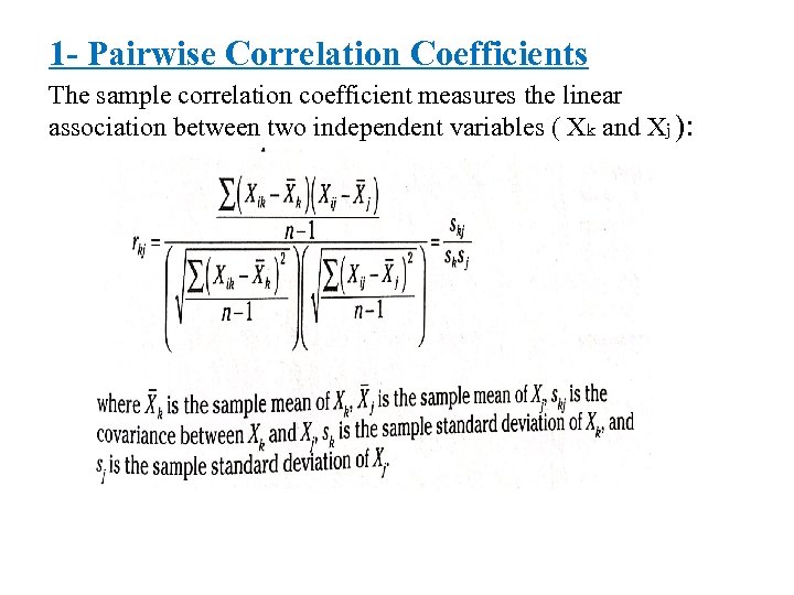1 - Pairwise Correlation Coefficients The sample correlation coefficient measures the linear association between two independent variables ( Xk and Xj ):

Ø The correlation matrix contains the correlation coefficients (ranges from 0 to |1| ) for each pair of independent variables. Ø As a result , correlation coefficients around 0. 8 or above may signal a multicollinearity problom. Ø Of course, before offically determing the multicollinearity problem, you should check your results for evidence of multicollinearity ( insignificant t-statistic, sensitive coefficient estimates, and nonsensical coefficient signs and values).

Ø Lower correlation coefficients do not necessairly indicate that you are a clear of multicollinearity. Ø The pairwise correlation coefficients only identify the linear relationship of a variable with one other variable.

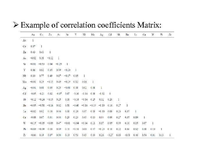Ø Example of correlation coefficients Matrix:

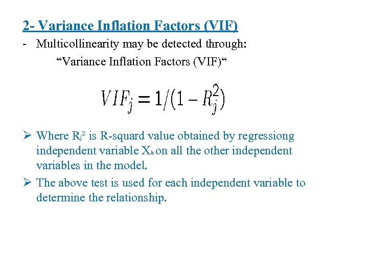2 - Variance Inflation Factors (VIF) - Multicollinearity may be detected through: “Variance Inflation Factors (VIF)“ Ø Where Rj² is R-squard value obtained by regressiong independent variable Xk on all the other independent variables in the model. Ø The above test is used for each independent variable to determine the relationship.

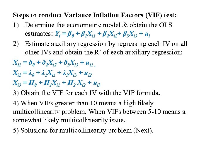Steps to conduct Variance Inflation Factors (VIF) test: 1) Determine the econometric model & obtain the OLS estimates: Yi = β 0 + β 1 Xi 1 + β 2 Xi 2+ β 3 Xi 3 + ui 2) Estimate auxiliary regression by regressing each IV on all other IVs and obtain the R² of each auxiliary regression: Xi 1 = ծ 0 + ծ 2 Xi 2 + ծ 3 Xi 3 + ui 1 , Xi 2 = λ 0 + λ 1 Xi 1 + λ 3 Xi 3 + ui 2 Xi 3 = Π 0 + Π 1 Xi 1 + Π 2 Xi 2 + ui 3 3) Obtain the VIF for each IV with the VIF formula. 4) When VIFs greater than 10 means a high likely multicollinearity problem. When VIFs between 5 -10 means a somewhat likely multicollinearity issue. 5) Solusions for multicollinearity problem (Next).

V. Resolve Multicollinearity Issues § Get more data: Gathering additional data not only improves the quality with your data but also helps with multicollinearity as it is a problem that related to the sample it self.

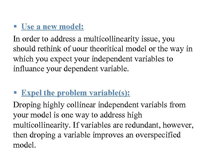§ Use a new model: In order to address a multicollinearity issue, you should rethink of uour theoritical model or the way in which you expect your independent variables to influance your dependent variable. § Expel the problem variable(s): Droping highly collinear independent variabls from your model is one way to address high multicollinearity. If variables are redundant, however, then droping a variable improves an overspecified model.