Econometrics 2 — Lecture 2 Models with Limited

Скачать презентацию Econometrics 2 — Lecture 2 Models with Limited

c83431131ddfe880b6e1cd92efacf2be.ppt

Количество слайдов: 96

Econometrics 2 - Lecture 2 Models with Limited Dependent Variables

Contents n n n Limited Dependent Variable Cases Binary Choice Models: Estimation Binary Choice Models: Goodness of Fit Application to Latent Models Multi-response Models Multinomial Models Count Data Models The Tobit Model: Estimation The Tobit II Model Mar 18, 2016 Hackl, Econometrics 2, Lecture 2 2

Example Explain whether a household owns a car: explanatory power have n income n household size n etc. Regression for describing car-ownership is not suitable! n Owning a car has two manifestations: yes/no n Indicator for owning a car is a binary variable Models are needed that allow to describe a binary dependent variable or a, more generally, limited dependent variable Mar 18, 2016 Hackl, Econometrics 2, Lecture 2 3

Cases of Limited Dependent Variables Typical situations: functions of explanatory variables are used to describe or explain n Dichotomous or binary dependent variable, e. g. , ownership of a car (yes/no), employment status (employed/unemployed), etc. n Ordered response, e. g. , qualitative assessment (good/average/bad), working status (full-time/part-time/not working), etc. n Multinomial response, e. g. , trading destinations (Europe/Asia/Africa), transportation means (train/bus/car), etc. n Count data, e. g. , number of orders a company receives in a week, number of patents granted to a company in a year n Censored data, e. g. , expenditures for durable goods, duration of study with drop outs Mar 18, 2016 Hackl, Econometrics 2, Lecture 2 4

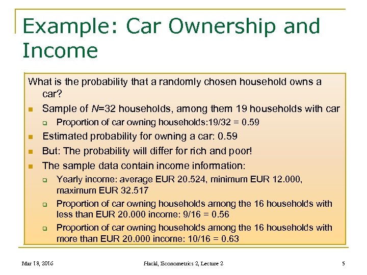Example: Car Ownership and Income What is the probability that a randomly chosen household owns a car? n Sample of N=32 households, among them 19 households with car q n n n Proportion of car owning households: 19/32 = 0. 59 Estimated probability for owning a car: 0. 59 But: The probability will differ for rich and poor! The sample data contain income information: q q q Mar 18, 2016 Yearly income: average EUR 20. 524, minimum EUR 12. 000, maximum EUR 32. 517 Proportion of car owning households among the 16 households with less than EUR 20. 000 income: 9/16 = 0. 56 Proportion of car owning households among the 16 households with more than EUR 20. 000 income: 10/16 = 0. 63 Hackl, Econometrics 2, Lecture 2 5

Car Ownership and Income, cont’d How can a model for the probability – or prediction – of car ownership take the income of a household into account? Notation: N households q q dummy yi for car ownership; yi =1: household i has car income of i-th household: xi 2 For predicting yi – or estimating the probability P{yi =1} – , a model is needed that takes the income into account Mar 18, 2016 Hackl, Econometrics 2, Lecture 2 6

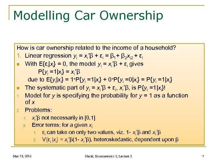Modelling Car Ownership How is car ownership related to the income of a household? 1. Linear regression yi = xi’β + εi = β 1+ β 2 xi 2 + εi n With E{εi|xi} = 0, the model yi = xi’β + εi gives P{yi =1|xi} = xi’β due to E{yi|xi} = 1*P{yi =1|xi} + 0*P{yi =0|xi} = P{yi =1|xi} n The systematic part of yi = xi’β + εi, xi’β, is P{yi =1|xi}! 1. Model for y is specifying the probability for y = 1 as a function of x 2. Problems: 1. 2. Mar 18, 2016 xi’β not necessarily in [0, 1] Error terms: for a given xi 1. εi can take on only two values, viz. 1 - xi’β and xi’β 2. V{εi |xi} = xi’β(1 - xi’β), heteroskedastic, dependent upon β Hackl, Econometrics 2, Lecture 2 7

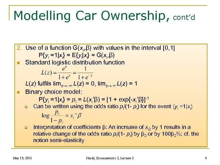Modelling Car Ownership, cont’d 2. Use of a function G(xi, β) with values in the interval [0, 1] P{yi =1|xi} = E{yi|xi} = G(xi, β) n Standard logistic distribution function n L(z) fulfils limz→ -∞ L(z) = 0, limz→ ∞ L(z) = 1 Binary choice model: P{yi =1|xi} = pi = L(xi’β) = [1 + exp{-xi’β}]-1 q q Mar 18, 2016 Can be written using the odds ratio pi/(1 - pi) for the event {yi =1|xi} Interpretation of coefficients β: An increase of xi 2 by 1 results in a relative change of the odds ratio pi/(1 - pi) by β 2 or by 100β 2%; cf. the notion semi-elasticity Hackl, Econometrics 2, Lecture 2 8

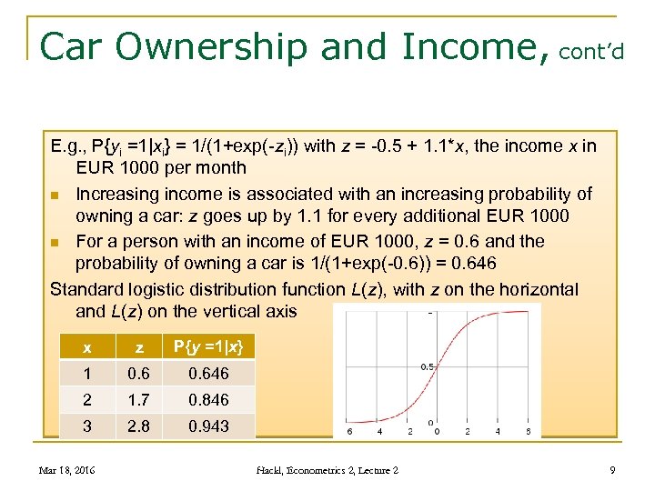Car Ownership and Income, cont’d E. g. , P{yi =1|xi} = 1/(1+exp(-zi)) with z = -0. 5 + 1. 1*x, the income x in EUR 1000 per month n Increasing income is associated with an increasing probability of owning a car: z goes up by 1. 1 for every additional EUR 1000 n For a person with an income of EUR 1000, z = 0. 6 and the probability of owning a car is 1/(1+exp(-0. 6)) = 0. 646 Standard logistic distribution function L(z), with z on the horizontal and L(z) on the vertical axis x z P{y =1|x} 1 0. 646 2 1. 7 0. 846 3 2. 8 0. 943 Mar 18, 2016 Hackl, Econometrics 2, Lecture 2 9

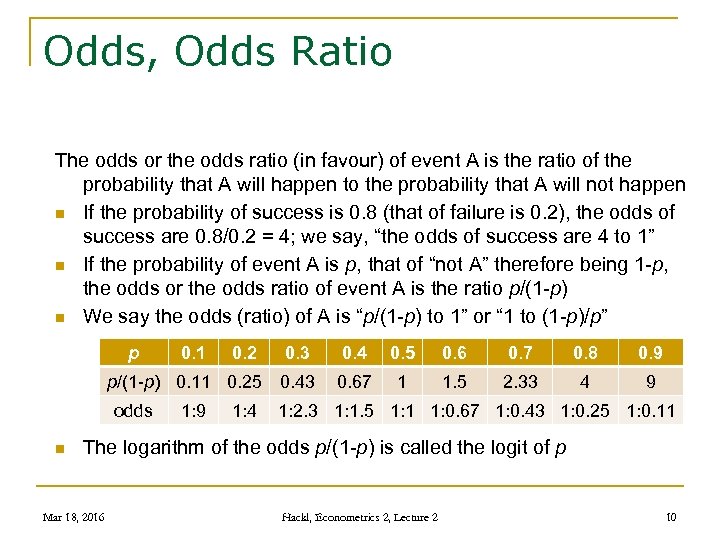Odds, Odds Ratio The odds or the odds ratio (in favour) of event A is the ratio of the probability that A will happen to the probability that A will not happen n If the probability of success is 0. 8 (that of failure is 0. 2), the odds of success are 0. 8/0. 2 = 4; we say, “the odds of success are 4 to 1” n If the probability of event A is p, that of “not A” therefore being 1 -p, the odds or the odds ratio of event A is the ratio p/(1 -p) n We say the odds (ratio) of A is “p/(1 -p) to 1” or “ 1 to (1 -p)/p” p 0. 2 0. 3 0. 4 0. 5 0. 6 0. 7 0. 8 0. 9 p/(1 -p) 0. 11 0. 25 0. 43 0. 67 1 1. 5 2. 33 4 9 odds n 0. 1 1: 9 1: 4 1: 2. 3 1: 1. 5 1: 1 1: 0. 67 1: 0. 43 1: 0. 25 1: 0. 11 The logarithm of the odds p/(1 -p) is called the logit of p Mar 18, 2016 Hackl, Econometrics 2, Lecture 2 10

Betting Odds n n n The probability of success is 0. 8 The odds of success are 4 to 1 Betting odds for success are 1: 4 q Mar 18, 2016 The bookmaker is prepared to pay out a prize of one fourth of the stake and return the stake as well, to anyone who places a bet on success Hackl, Econometrics 2, Lecture 2 11

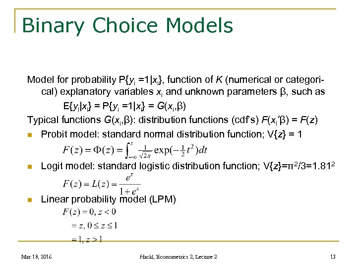Binary Choice Models Model for probability P{yi =1|xi}, function of K (numerical or categorical) explanatory variables xi and unknown parameters β, such as E{yi|xi} = P{yi =1|xi} = G(xi, β) Typical functions G(xi, β): distribution functions (cdf’s) F(xi’β) = F(z) n Probit model: standard normal distribution function; V{z} = 1 n Logit model: standard logistic distribution function; V{z}=π2/3=1. 812 n Linear probability model (LPM) Mar 18, 2016 Hackl, Econometrics 2, Lecture 2 13

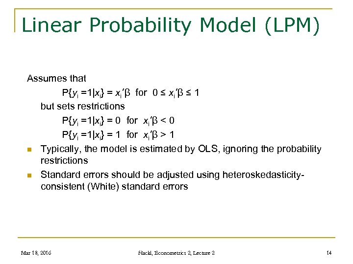Linear Probability Model (LPM) Assumes that P{yi =1|xi} = xi’β for 0 ≤ xi’β ≤ 1 but sets restrictions P{yi =1|xi} = 0 for xi’β < 0 P{yi =1|xi} = 1 for xi’β > 1 n Typically, the model is estimated by OLS, ignoring the probability restrictions n Standard errors should be adjusted using heteroskedasticityconsistent (White) standard errors Mar 18, 2016 Hackl, Econometrics 2, Lecture 2 14

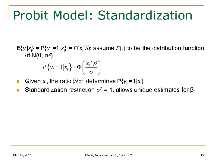Probit Model: Standardization E{yi|xi} = P{yi =1|xi} = F(xi’β): assume F(. ) to be the distribution function of N(0, σ2) n n Given xi, the ratio β/σ2 determines P{yi =1|xi} Standardization restriction 2 = 1: allows unique estimates for β Mar 18, 2016 Hackl, Econometrics 2, Lecture 2 15

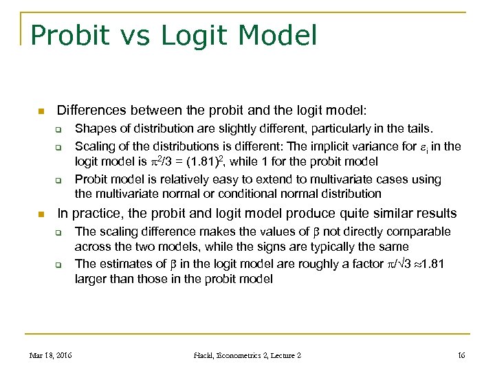Probit vs Logit Model n Differences between the probit and the logit model: q q q n Shapes of distribution are slightly different, particularly in the tails. Scaling of the distributions is different: The implicit variance for i in the logit model is 2/3 = (1. 81)2, while 1 for the probit model Probit model is relatively easy to extend to multivariate cases using the multivariate normal or conditional normal distribution In practice, the probit and logit model produce quite similar results q q Mar 18, 2016 The scaling difference makes the values of not directly comparable across the two models, while the signs are typically the same The estimates of in the logit model are roughly a factor / 3 1. 81 larger than those in the probit model Hackl, Econometrics 2, Lecture 2 16

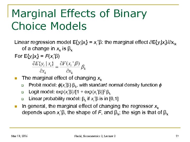Marginal Effects of Binary Choice Models Linear regression model E{yi|xi} = xi’β: the marginal effect E{yi|xi}/ xik of a change in xk is βk For E{yi|xi} = F(xi’β) n The marginal effect of changing xk q q q n Probit model: ϕ(xi’β) βk, with standard normal density function ϕ Logit model: exp{xi’β}/[1 + exp{xi’β}]2 βk Linear probability model: βk if xi’β is in [0, 1] In general, the marginal effect of changing the regressor xk depends upon xi’β, the shape of F, and βk; the sign is that of βk Mar 18, 2016 Hackl, Econometrics 2, Lecture 2 17

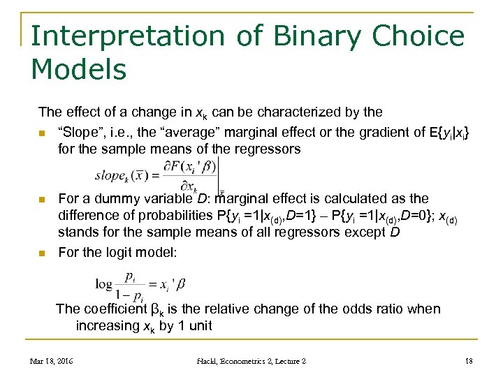Interpretation of Binary Choice Models The effect of a change in xk can be characterized by the n “Slope”, i. e. , the “average” marginal effect or the gradient of E{yi|xi} for the sample means of the regressors n n For a dummy variable D: marginal effect is calculated as the difference of probabilities P{yi =1|x(d), D=1} – P{yi =1|x(d), D=0}; x(d) stands for the sample means of all regressors except D For the logit model: The coefficient βk is the relative change of the odds ratio when increasing xk by 1 unit Mar 18, 2016 Hackl, Econometrics 2, Lecture 2 18

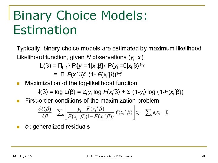Binary Choice Models: Estimation Typically, binary choice models are estimated by maximum likelihood Likelihood function, given N observations (yi, xi) L(β) = Πi=1 N P{yi =1|xi; β}yi P{yi =0|xi; β}1 -yi = Πi F(xi’β)yi (1 - F(xi’β))1 -yi n Maximization of the log-likelihood function ℓ(β) = log L(β) = Si yi log F(xi’β) + Si (1 -yi) log (1 -F(xi’β)) n First-order conditions of the maximization problem n ei: generalized residuals Mar 18, 2016 Hackl, Econometrics 2, Lecture 2 20

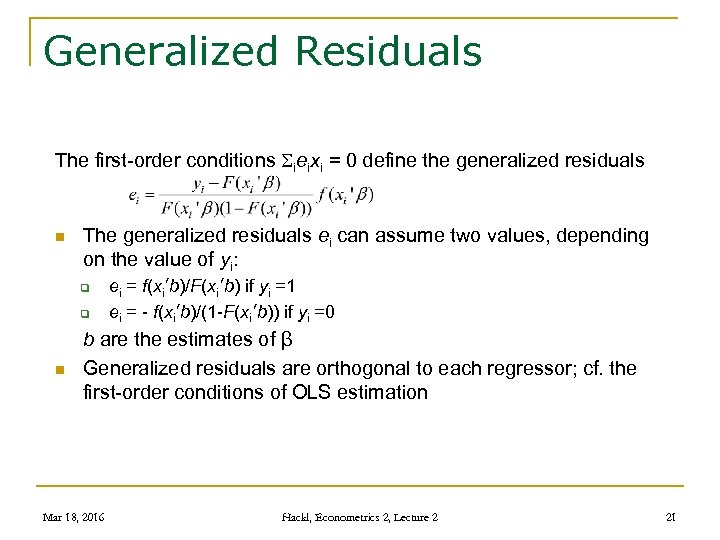Generalized Residuals The first-order conditions Sieixi = 0 define the generalized residuals n The generalized residuals ei can assume two values, depending on the value of yi: q q n ei = f(xi’b)/F(xi’b) if yi =1 ei = - f(xi’b)/(1 -F(xi’b)) if yi =0 b are the estimates of β Generalized residuals are orthogonal to each regressor; cf. the first-order conditions of OLS estimation Mar 18, 2016 Hackl, Econometrics 2, Lecture 2 21

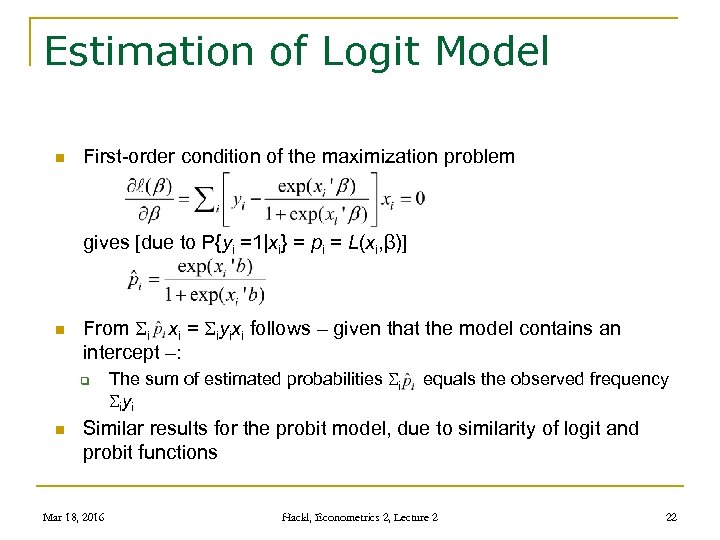Estimation of Logit Model n First-order condition of the maximization problem gives [due to P{yi =1|xi} = pi = L(xi, β)] n From Si xi = Siyixi follows – given that the model contains an intercept –: q n The sum of estimated probabilities Si equals the observed frequency Siyi Similar results for the probit model, due to similarity of logit and probit functions Mar 18, 2016 Hackl, Econometrics 2, Lecture 2 22

Binary Choice Models in GRETL Model > Nonlinear Models > Logit > Binary Estimates the specified model using error terms with standard logistic distribution Model > Nonlinear Models > Probit > Binary n n Estimates the specified model using error terms with standard normal distribution Mar 18, 2016 Hackl, Econometrics 2, Lecture 2 23

Example: Effect of Teaching Method Study by Spector & Mazzeo (1980); see Greene (2003), Chpt. 21 Personalized System of Instruction: a new teaching method in economics; has it an effect on student performance in later courses? n Data: q q n GRADE (0/1): indicator whether grade was higher than in principal course PSI (0/1): participation in program with new teaching method GPA: grade point average TUCE: score on a pre-test, entering knowledge 32 observations mean min max GPA 2. 06 4. 00 TUCE Mar 18, 2016 3. 12 21. 9 12 29 Hackl, Econometrics 2, Lecture 2 24

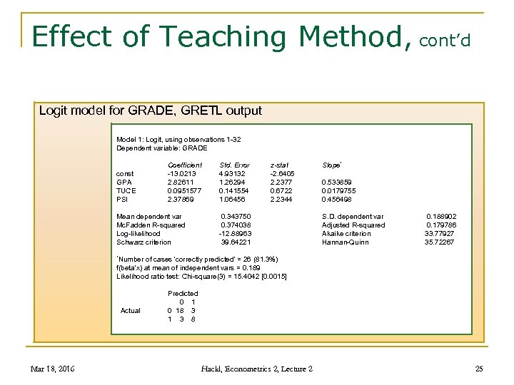Effect of Teaching Method, cont’d Logit model for GRADE, GRETL output Model 1: Logit, using observations 1 -32 Dependent variable: GRADE const GPA TUCE PSI Coefficient -13. 0213 2. 82611 0. 0951577 2. 37869 Mean dependent var Mc. Fadden R-squared Log-likelihood Schwarz criterion Std. Error 4. 93132 1. 26294 0. 141554 1. 06456 z-stat -2. 6405 2. 2377 0. 6722 2. 2344 0. 343750 0. 374038 -12. 88963 39. 64221 Slope* 0. 533859 0. 0179755 0. 456498 S. D. dependent var Adjusted R-squared Akaike criterion Hannan-Quinn 0. 188902 0. 179786 33. 77927 35. 72267 *Number of cases 'correctly predicted' = 26 (81. 3%) f(beta'x) at mean of independent vars = 0. 189 Likelihood ratio test: Chi-square(3) = 15. 4042 [0. 0015] Actual Mar 18, 2016 Predicted 0 1 0 18 3 1 3 8 Hackl, Econometrics 2, Lecture 2 25

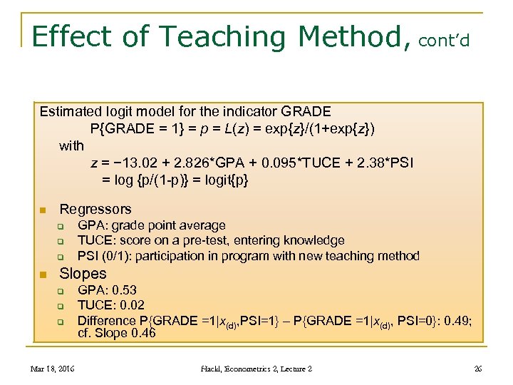Effect of Teaching Method, cont’d Estimated logit model for the indicator GRADE P{GRADE = 1} = p = L(z) = exp{z}/(1+exp{z}) with z = − 13. 02 + 2. 826*GPA + 0. 095*TUCE + 2. 38*PSI = log {p/(1 -p)} = logit{p} n Regressors q q q n GPA: grade point average TUCE: score on a pre-test, entering knowledge PSI (0/1): participation in program with new teaching method Slopes q q q Mar 18, 2016 GPA: 0. 53 TUCE: 0. 02 Difference P{GRADE =1|x(d), PSI=1} – P{GRADE =1|x(d), PSI=0}: 0. 49; cf. Slope 0. 46 Hackl, Econometrics 2, Lecture 2 26

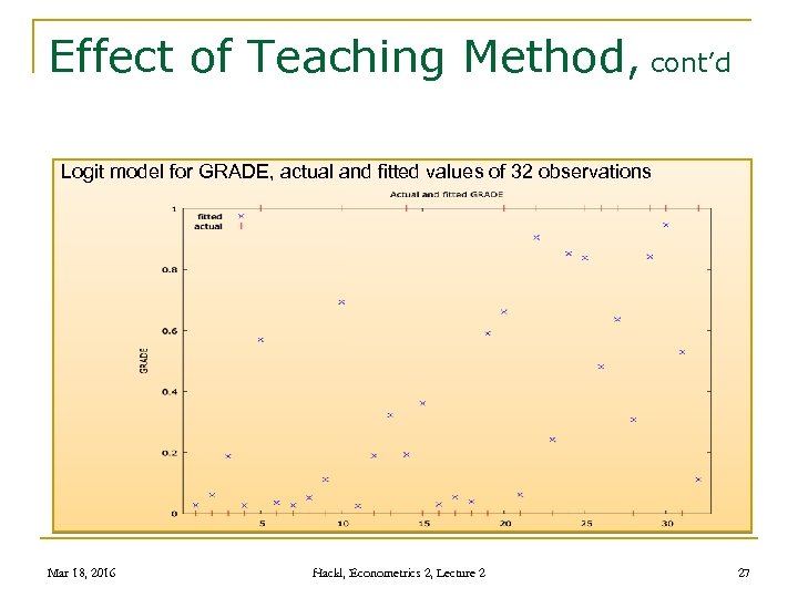Effect of Teaching Method, cont’d Logit model for GRADE, actual and fitted values of 32 observations Mar 18, 2016 Hackl, Econometrics 2, Lecture 2 27

Properties of ML Estimators Consistent n Asymptotically efficient n Asymptotically normally distributed These properties require that the assumed distribution is correct n Correct shape n No autocorrelation and/or heteroskedasticity n No dependence – correlations – between errors and regressors n No omitted regressors n Mar 18, 2016 Hackl, Econometrics 2, Lecture 2 28

Goodness-of-Fit Measures Concepts n Comparison of the maximum likelihood of the model with that of the naïve model, i. e. , a model with only an intercept, no regressors q q n pseudo-r 2 Mc. Fadden R 2 Index based on proportion of correctly predicted observations or hit rates q Mar 18, 2016 Rp 2 Hackl, Econometrics 2, Lecture 2 30

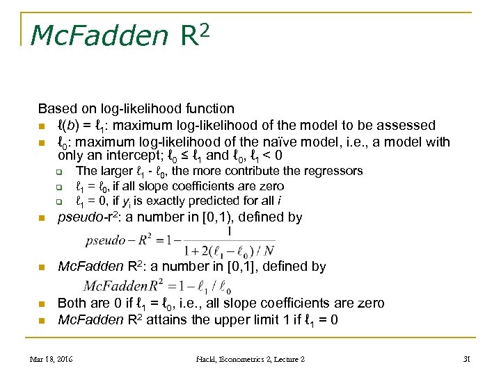Mc. Fadden R 2 Based on log-likelihood function n ℓ(b) = ℓ 1: maximum log-likelihood of the model to be assessed n ℓ 0: maximum log-likelihood of the naïve model, i. e. , a model with only an intercept; ℓ 0 ≤ ℓ 1 and ℓ 0, ℓ 1 < 0 q q q The larger ℓ 1 - ℓ 0, the more contribute the regressors ℓ 1 = ℓ 0, if all slope coefficients are zero ℓ 1 = 0, if yi is exactly predicted for all i n pseudo-r 2: a number in [0, 1), defined by n Mc. Fadden R 2: a number in [0, 1], defined by n Both are 0 if ℓ 1 = ℓ 0, i. e. , all slope coefficients are zero Mc. Fadden R 2 attains the upper limit 1 if ℓ 1 = 0 n Mar 18, 2016 Hackl, Econometrics 2, Lecture 2 31

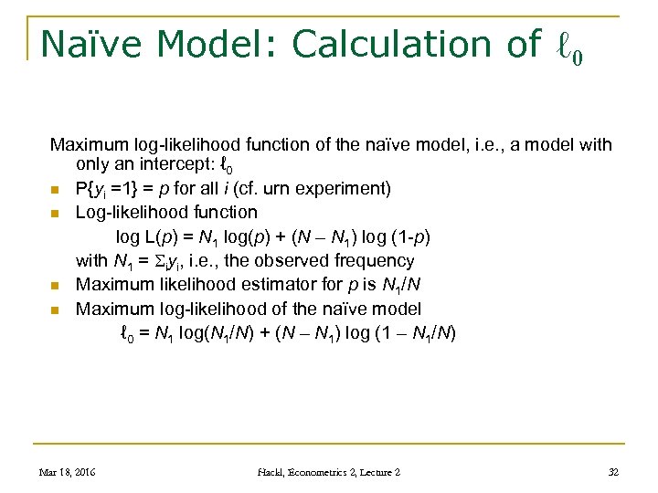Naïve Model: Calculation of ℓ 0 Maximum log-likelihood function of the naïve model, i. e. , a model with only an intercept: ℓ 0 n P{yi =1} = p for all i (cf. urn experiment) n Log-likelihood function log L(p) = N 1 log(p) + (N – N 1) log (1 -p) with N 1 = Siyi, i. e. , the observed frequency n Maximum likelihood estimator for p is N 1/N n Maximum log-likelihood of the naïve model ℓ 0 = N 1 log(N 1/N) + (N – N 1) log (1 – N 1/N) Mar 18, 2016 Hackl, Econometrics 2, Lecture 2 32

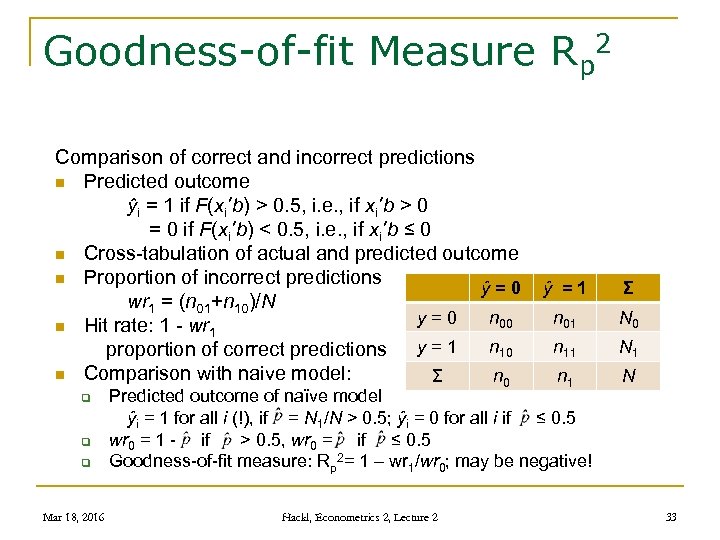Goodness-of-fit Measure Rp 2 Comparison of correct and incorrect predictions n Predicted outcome ŷi = 1 if F(xi’b) > 0. 5, i. e. , if xi’b > 0 = 0 if F(xi’b) < 0. 5, i. e. , if xi’b ≤ 0 n Cross-tabulation of actual and predicted outcome n Proportion of incorrect predictions ŷ=0 wr 1 = (n 01+n 10)/N y = 0 n 00 n Hit rate: 1 - wr 1 n 10 proportion of correct predictions y = 1 n Comparison with naive model: Σ n 0 q q q Mar 18, 2016 ŷ =1 Σ n 01 N 0 n 11 N 1 n 1 N Predicted outcome of naïve model ŷi = 1 for all i (!), if = N 1/N > 0. 5; ŷi = 0 for all i if ≤ 0. 5 wr 0 = 1 - if > 0. 5, wr 0 = if ≤ 0. 5 Goodness-of-fit measure: Rp 2= 1 – wr 1/wr 0; may be negative! Hackl, Econometrics 2, Lecture 2 33

Example: Effect of Teaching Method Study by Spector & Mazzeo (1980); see Greene (2003), Chpt. 21 Personalized System of Instruction: new teaching method in economics; has it an effect on student performance in later courses? n Data: q q n GRADE (0/1): indicator whether grade was higher than in principal course PSI (0/1): participation in program with new teaching method GPA: grade point average TUCE: score on a pre-test, entering knowledge 32 observations Mar 18, 2016 Hackl, Econometrics 2, Lecture 2 34

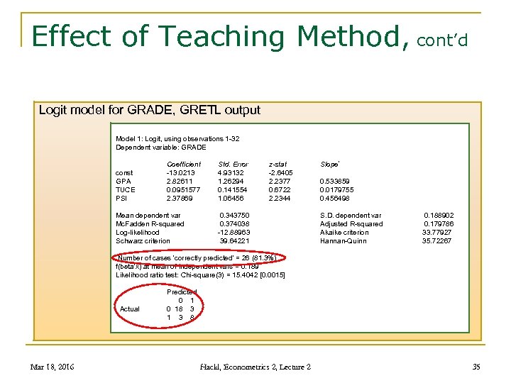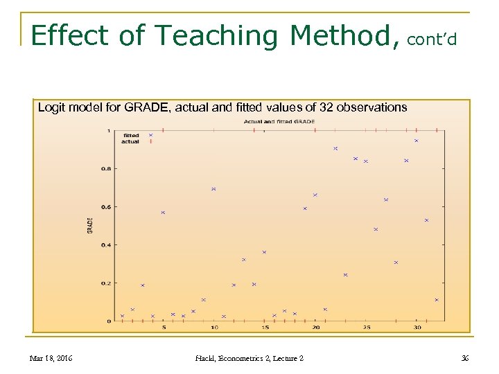Effect of Teaching Method, cont’d Logit model for GRADE, actual and fitted values of 32 observations Mar 18, 2016 Hackl, Econometrics 2, Lecture 2 36

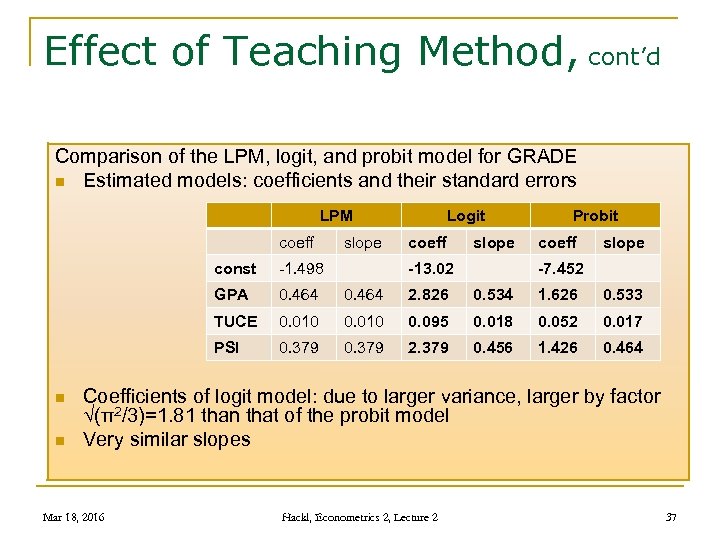Effect of Teaching Method, cont’d Comparison of the LPM, logit, and probit model for GRADE n Estimated models: coefficients and their standard errors LPM coeff slope Logit coeff slope const 0. 464 2. 826 0. 534 1. 626 0. 533 TUCE 0. 010 0. 095 0. 018 0. 052 0. 017 PSI n -1. 498 GPA n -13. 02 Probit -7. 452 0. 379 2. 379 0. 456 1. 426 0. 464 Coefficients of logit model: due to larger variance, larger by factor √(π2/3)=1. 81 than that of the probit model Very similar slopes Mar 18, 2016 Hackl, Econometrics 2, Lecture 2 37

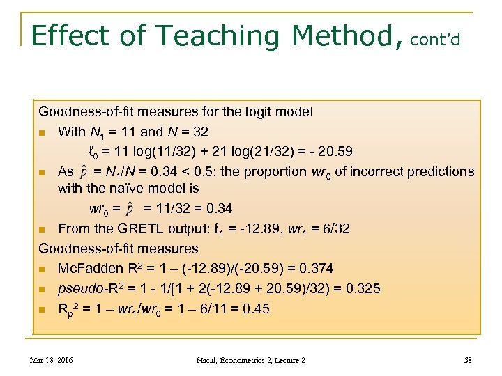Effect of Teaching Method, cont’d Goodness-of-fit measures for the logit model n With N 1 = 11 and N = 32 ℓ 0 = 11 log(11/32) + 21 log(21/32) = - 20. 59 n As = N 1/N = 0. 34 < 0. 5: the proportion wr 0 of incorrect predictions with the naïve model is wr 0 = = 11/32 = 0. 34 n From the GRETL output: ℓ 1 = -12. 89, wr 1 = 6/32 Goodness-of-fit measures n Mc. Fadden R 2 = 1 – (-12. 89)/(-20. 59) = 0. 374 n pseudo-R 2 = 1 - 1/[1 + 2(-12. 89 + 20. 59)/32) = 0. 325 n Rp 2 = 1 – wr 1/wr 0 = 1 – 6/11 = 0. 45 Mar 18, 2016 Hackl, Econometrics 2, Lecture 2 38

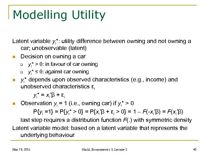Modelling Utility Latent variable yi*: utility difference between owning and not owning a car; unobservable (latent) n Decision on owning a car q q yi* > 0: in favour of car owning yi* ≤ 0: against car owning yi* depends upon observed characteristics (e. g. , income) and unobserved characteristics εi yi* = xi’β + εi n Observation yi = 1 (i. e. , owning car) if yi* > 0 P{yi =1} = P{yi* > 0} = P{xi’β + εi > 0} = 1 – F(-xi’β) = F(xi’β) last step requires a distribution function F(. ) with symmetric density Latent variable model: based on a latent variable that represents the underlying behaviour n Mar 18, 2016 Hackl, Econometrics 2, Lecture 2 40

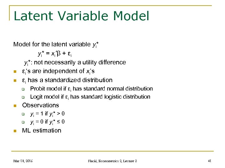Latent Variable Model for the latent variable yi* = xi’β + εi yi*: not necessarily a utility difference n εi‘s are independent of xi’s n εi has a standardized distribution q q n Observations q q n Probit model if εi has standard normal distribution Logit model if εi has standard logistic distribution yi = 1 if yi* > 0 yi = 0 if yi* ≤ 0 ML estimation Mar 18, 2016 Hackl, Econometrics 2, Lecture 2 41

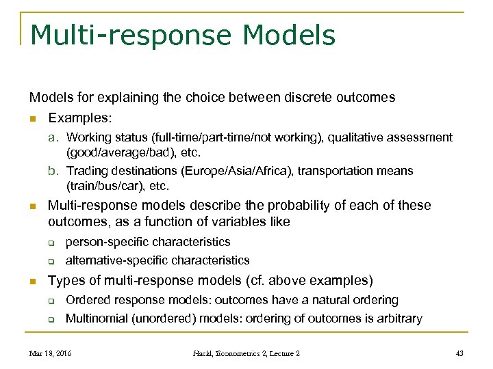Multi-response Models for explaining the choice between discrete outcomes n Examples: a. Working status (full-time/part-time/not working), qualitative assessment (good/average/bad), etc. b. Trading destinations (Europe/Asia/Africa), transportation means (train/bus/car), etc. n Multi-response models describe the probability of each of these outcomes, as a function of variables like q q n person-specific characteristics alternative-specific characteristics Types of multi-response models (cf. above examples) q Ordered response models: outcomes have a natural ordering q Multinomial (unordered) models: ordering of outcomes is arbitrary Mar 18, 2016 Hackl, Econometrics 2, Lecture 2 43

Example: Credit Rating Credit rating: numbers, indicating experts’ opinion about (a firm’s) capacity to satisfy financial obligations, e. g. , credit-worthiness n n Standard & Poor's rating scale: AAA, AA+, AA-, A+, A, A-, BBB+, BBB-, BB+, BB-, B+, B, B-, CCC+, CCC-, CC, C, D Verbeek‘s data set CREDIT q q n Categories “ 1“, …, “ 7“ (highest) Investment grade with alternatives “ 1” (better than category 3) and “ 0” (category 3 or less, also called “speculative grade“) Explanatory variables, e. g. , q Firm sales q Ebit, i. e. , earnings before interest and taxes q Ratio of working capital to total assets Mar 18, 2016 Hackl, Econometrics 2, Lecture 2 44

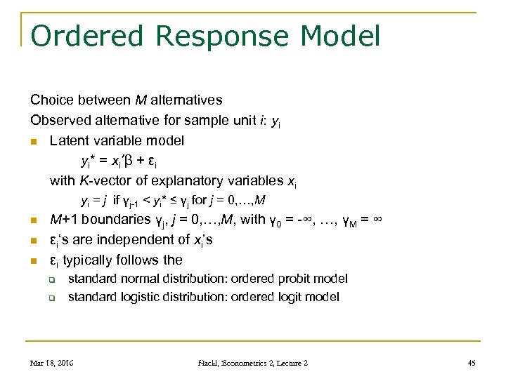Ordered Response Model Choice between M alternatives Observed alternative for sample unit i: yi n Latent variable model yi* = xi’β + εi with K-vector of explanatory variables xi yi = j if γj-1 < yi* ≤ γj for j = 0, …, M n n n M+1 boundaries γj, j = 0, …, M, with γ 0 = -∞, …, γM = ∞ εi‘s are independent of xi’s εi typically follows the q q standard normal distribution: ordered probit model standard logistic distribution: ordered logit model Mar 18, 2016 Hackl, Econometrics 2, Lecture 2 45

Example: Willingness to Work Married females are asked: „How much would you like to work? “ Potential answers of individual i: yi = 1 (not working), yi = 2 (part time), yi = 3 (full time) n Measure of the desired labour supply n Dependent upon factors like age, education level, husband‘s income Ordered response model with M = 3 yi* = xi’β + εi with yi = 1 if yi* ≤ 0 yi = 2 if 0 < yi* ≤ γ yi = 3 if yi* > γ n n εi‘s with distribution function F(. ) yi* stands for “willingness to work” or “desired hours of work” Mar 18, 2016 Hackl, Econometrics 2, Lecture 2 46

Willingness to Work, cont’d In terms of observed quantities: P{yi = 1 |xi} = P{yi* ≤ 0 |xi} = F(- xi’β) P{yi = 3 |xi} = P{yi* > γ |xi} = 1 - F(γ - xi’β) P{yi = 2 |xi} = F(γ - xi’β) – F(- xi’β) n Unknown parameters: γ and β n Standardization: wrt location (γ = 0) and scale (V{εi} = 1) n ML estimation Interpretation of parameters β n Wrt yi*(= xi’β + εi): willingness to work increases with larger xk for positive βk n Wrt probabilities P{yi = j |xi}, e. g. , for positive βk q q P{yi = 3 |xi} = P{yi* > γ |xi} increases and P{yi = 1 |xi} P{yi* ≤ 0 |xi} decreases with larger xk Mar 18, 2016 Hackl, Econometrics 2, Lecture 2 47

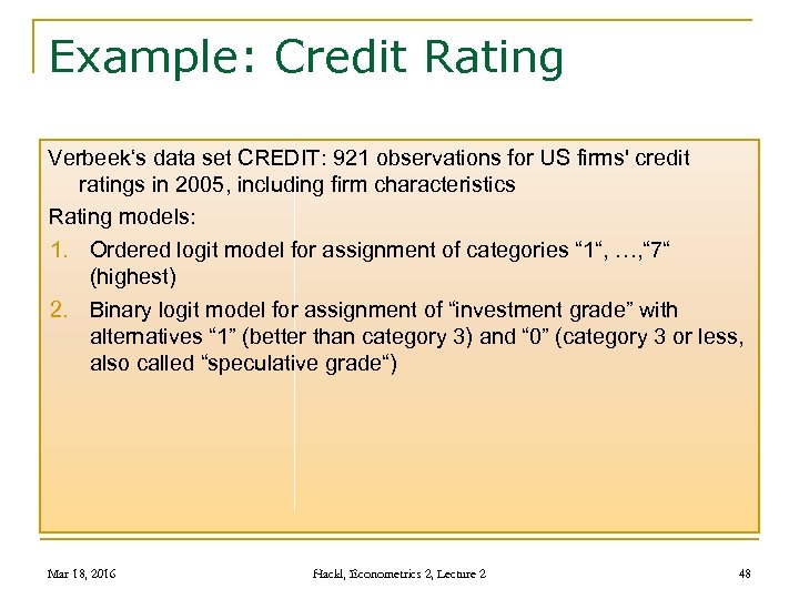Example: Credit Rating Verbeek‘s data set CREDIT: 921 observations for US firms' credit ratings in 2005, including firm characteristics Rating models: 1. Ordered logit model for assignment of categories “ 1“, …, “ 7“ (highest) 2. Binary logit model for assignment of “investment grade” with alternatives “ 1” (better than category 3) and “ 0” (category 3 or less, also called “speculative grade“) Mar 18, 2016 Hackl, Econometrics 2, Lecture 2 48

Credit Rating, cont’d Verbeek‘s data set CREDIT Ratings and characteristics for 921 firms: summary statistics ___________ Book leverage: ratio of debts to assets Mar 18, 2016 Hackl, Econometrics 2, Lecture 2 49

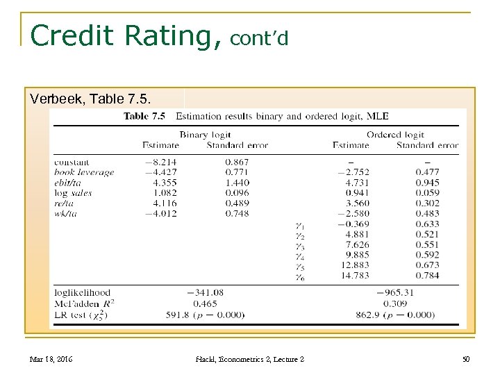Credit Rating, cont’d Verbeek, Table 7. 5. Mar 18, 2016 Hackl, Econometrics 2, Lecture 2 50

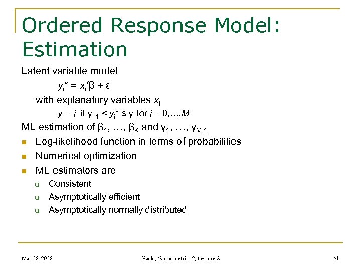Ordered Response Model: Estimation Latent variable model yi* = xi’β + εi with explanatory variables xi yi = j if γj-1 < yi* ≤ γj for j = 0, …, M ML estimation of β 1, …, βK and γ 1, …, γM-1 n Log-likelihood function in terms of probabilities n Numerical optimization n ML estimators are q q q Consistent Asymptotically efficient Asymptotically normally distributed Mar 18, 2016 Hackl, Econometrics 2, Lecture 2 51

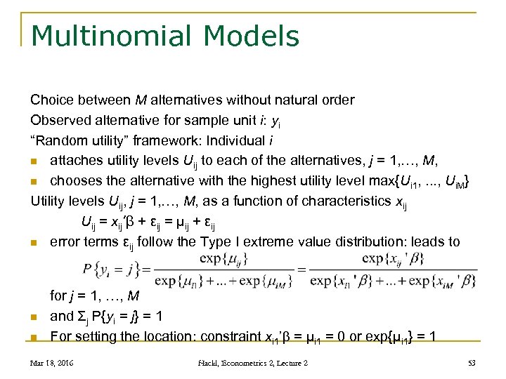Multinomial Models Choice between M alternatives without natural order Observed alternative for sample unit i: yi “Random utility” framework: Individual i n attaches utility levels Uij to each of the alternatives, j = 1, …, M, n chooses the alternative with the highest utility level max{Ui 1, . . . , Ui. M} Utility levels Uij, j = 1, …, M, as a function of characteristics xij Uij = xij’β + εij = μij + εij n error terms εij follow the Type I extreme value distribution: leads to n n for j = 1, …, M and Σj P{yi = j} = 1 For setting the location: constraint xi 1’ = μi 1 = 0 or exp{μi 1} = 1 Mar 18, 2016 Hackl, Econometrics 2, Lecture 2 53

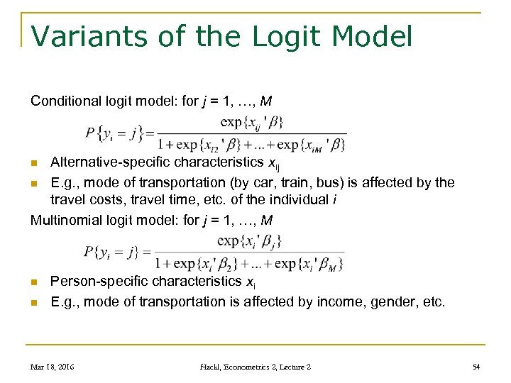Variants of the Logit Model Conditional logit model: for j = 1, …, M Alternative-specific characteristics xij n E. g. , mode of transportation (by car, train, bus) is affected by the travel costs, travel time, etc. of the individual i Multinomial logit model: for j = 1, …, M n n n Person-specific characteristics xi E. g. , mode of transportation is affected by income, gender, etc. Mar 18, 2016 Hackl, Econometrics 2, Lecture 2 54

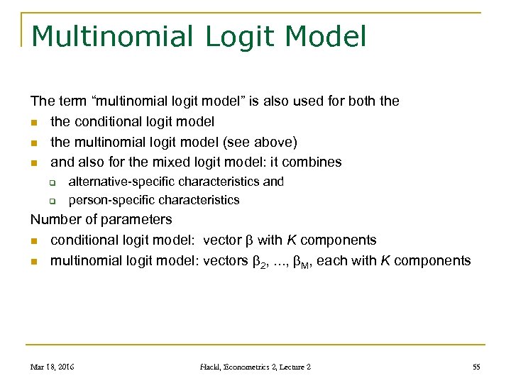Multinomial Logit Model The term “multinomial logit model” is also used for both the n the conditional logit model n the multinomial logit model (see above) n and also for the mixed logit model: it combines q q alternative-specific characteristics and person-specific characteristics Number of parameters n conditional logit model: vector with K components n multinomial logit model: vectors 2, . . . , M, each with K components Mar 18, 2016 Hackl, Econometrics 2, Lecture 2 55

Independence of Errors Independence of the error terms εij implies independent utility levels of alternatives n Independence assumption may be restrictive n Example: High utility of alternative „travel with red bus“ implies high utility of „travel with blue bus“ n Implies that the odds ratio of two alternatives does not depend upon other alternatives: “independence of irrelevant alternatives” (IIA) Mar 18, 2016 Hackl, Econometrics 2, Lecture 2 56

Multi-response Models in GRETL Model > Nonlinear Models > Logit > Ordered. . . Estimates the specified model using error terms with standard logistic distribution, assuming ordered alternatives for responses Model > Nonlinear Models > Logit > Multinomial. . . n Estimates the specified model using error terms with standard logistic distribution, assuming alternatives without order Model > Nonlinear Models > Probit > Ordered. . . n n Estimates the specified model using error terms with standard normal distribution, assuming ordered alternatives Mar 18, 2016 Hackl, Econometrics 2, Lecture 2 57

Models for Count Data Describe the number of times an event occurs, depending upon certain characteristics Examples: n Number of visits in the library per week n Number of visits of a customer in the supermarket n Number of misspellings in an email n Number of applications of a firm for a patent, as a function of q q Firm size R&D expenditures Industrial sector Country, etc. See Verbeek‘s data set PATENT Mar 18, 2016 Hackl, Econometrics 2, Lecture 2 59

Example: Patents and R&D Expenditures Verbeek‘s data set PATENTS: number of patents (p 91), expenditures for R&D (logrd 91), sector of industry, and region; N = 181 Question: Is the number of patents depending of R&D expenditures, sector, region? Mar 18, 2016 Hackl, Econometrics 2, Lecture 2 60

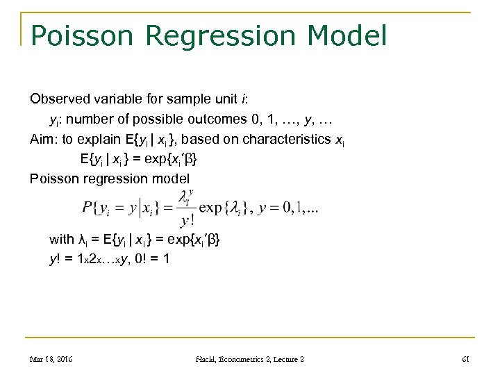Poisson Regression Model Observed variable for sample unit i: yi: number of possible outcomes 0, 1, …, y, … Aim: to explain E{yi | xi }, based on characteristics xi E{yi | xi } = exp{xi’β} Poisson regression model with λi = E{yi | xi } = exp{xi’β} y! = 1 x 2 x…xy, 0! = 1 Mar 18, 2016 Hackl, Econometrics 2, Lecture 2 61

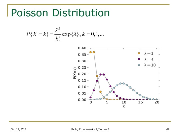Poisson Distribution Mar 18, 2016 Hackl, Econometrics 2, Lecture 2 62

Poisson Regression Model: Estimation Unknown parameters: coefficients β Estimates of β allow assessing how exp{xi’β} = E{yi | xi } is affected by xi Fitting the model to data: ML estimators for β are n Consistent n Asymptotically efficient n Asymptotically normally distributed Mar 18, 2016 Hackl, Econometrics 2, Lecture 2 63

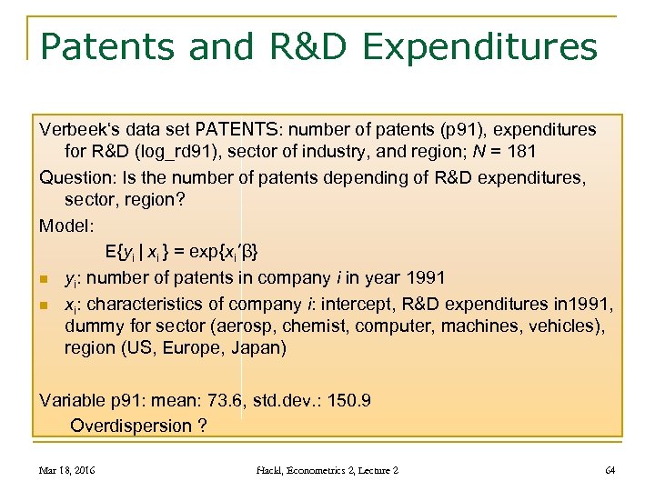Patents and R&D Expenditures Verbeek‘s data set PATENTS: number of patents (p 91), expenditures for R&D (log_rd 91), sector of industry, and region; N = 181 Question: Is the number of patents depending of R&D expenditures, sector, region? Model: E{yi | xi } = exp{xi’β} n yi: number of patents in company i in year 1991 n xi: characteristics of company i: intercept, R&D expenditures in 1991, dummy for sector (aerosp, chemist, computer, machines, vehicles), region (US, Europe, Japan) Variable p 91: mean: 73. 6, std. dev. : 150. 9 Overdispersion ? Mar 18, 2016 Hackl, Econometrics 2, Lecture 2 64

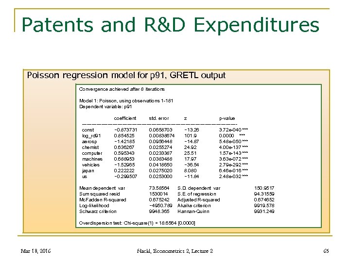Patents and R&D Expenditures Poisson regression model for p 91, GRETL output Convergence achieved after 8 iterations Model 1: Poisson, using observations 1 -181 Dependent variable: p 91 coefficient std. error z p-value ------------------------------------------------ const − 0. 873731 0. 0658703 − 13. 26 3. 72 e-040 *** log_rd 91 0. 854525 0. 00838674 101. 9 0. 0000 *** aerosp − 1. 42185 0. 0956448 − 14. 87 5. 48 e-050 *** chemist 0. 636267 0. 0255274 24. 92 4. 00 e-137 *** computer 0. 595343 0. 0233387 25. 51 1. 57 e-143 *** machines 0. 688953 0. 0383488 17. 97 3. 63 e-072 *** vehicles − 1. 52965 0. 0418650 − 36. 54 2. 79 e-292 *** japan 0. 222222 0. 0275020 8. 080 6. 46 e-016 *** us − 0. 299507 0. 0253000 − 11. 84 2. 48 e-032 *** Mean dependent var Sum squared resid Mc. Fadden R-squared Log-likelihood Schwarz criterion 73. 58564 S. D. dependent var 1530014 S. E. of regression 0. 675242 Adjusted R-squared − 4950. 789 Akaike criterion 9948. 365 Hannan-Quinn 150. 9517 94. 31559 0. 674652 9919. 578 9931. 249 Overdispersion test: Chi-square(1) = 18. 6564 [0. 0000] Mar 18, 2016 Hackl, Econometrics 2, Lecture 2 65

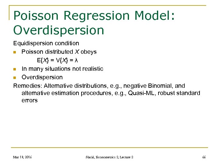Poisson Regression Model: Overdispersion Equidispersion condition n Poisson distributed X obeys E{X} = V{X} = λ n In many situations not realistic n Overdispersion Remedies: Alternative distributions, e. g. , negative Binomial, and alternative estimation procedures, e. g. , Quasi-ML, robust standard errors Mar 18, 2016 Hackl, Econometrics 2, Lecture 2 66

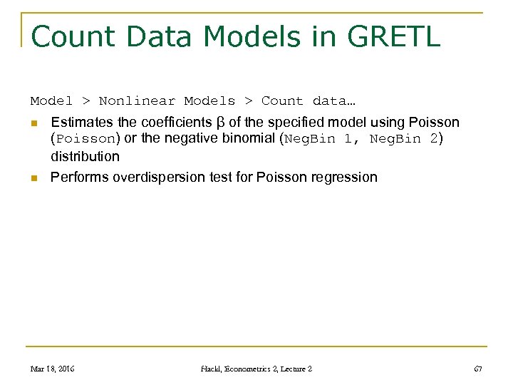Count Data Models in GRETL Model > Nonlinear Models > Count data… n n Estimates the coefficients β of the specified model using Poisson (Poisson) or the negative binomial (Neg. Bin 1, Neg. Bin 2) distribution Performs overdispersion test for Poisson regression Mar 18, 2016 Hackl, Econometrics 2, Lecture 2 67

Tobit Models Tobit models are regression models where the range of the (continuous) dependent variable is constrained, i. e. , censored from below Examples: n Hours of work as a function of age, qualification, etc. n Expenditures on alcoholic beverages and tobacco n Holiday expenditures as a function of the number of children n Expenditures on durable goods as a function of income, age, etc. : a part of units does not spend any money on durable goods Tobit models n Standard Tobit model or Tobit I model; James Tobin (1958) on expenditures on durable goods n Generalizations: Tobit II to V Mar 18, 2016 Hackl, Econometrics 2, Lecture 2 69

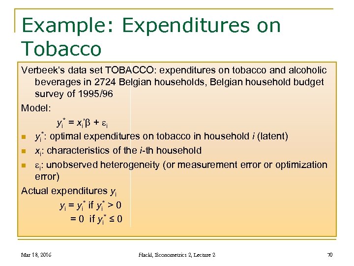Example: Expenditures on Tobacco Verbeek‘s data set TOBACCO: expenditures on tobacco and alcoholic beverages in 2724 Belgian households, Belgian household budget survey of 1995/96 Model: yi* = xi’ + i n yi*: optimal expenditures on tobacco in household i (latent) n xi: characteristics of the i-th household n i: unobserved heterogeneity (or measurement error or optimization error) Actual expenditures yi = yi* if yi* > 0 = 0 if yi* ≤ 0 Mar 18, 2016 Hackl, Econometrics 2, Lecture 2 70

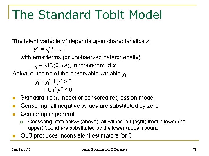The Standard Tobit Model The latent variable yi* depends upon characteristics xi yi* = xi’ + i with error terms (or unobserved heterogeneity) i ~ NID(0, 2), independent of xi Actual outcome of the observable variable yi = yi* if yi* > 0 = 0 if yi* ≤ 0 n Standard Tobit model or censored regression model n Censoring: all negative values are substituted by zero n Censoring in general q n Censoring from below (above): all values left (right) from a lower (an upper) bound are substituted by the lower (upper) bound OLS produces inconsistent estimators for Mar 18, 2016 Hackl, Econometrics 2, Lecture 2 71

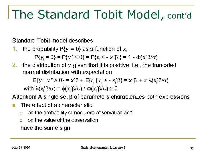The Standard Tobit Model, cont’d Standard Tobit model describes 1. the probability P{yi = 0} as a function of xi P{yi = 0} = P{yi* 0} = P{ i - xi’ } = 1 - (xi’ / ) 2. the distribution of yi given that it is positive, i. e. , the truncated normal distribution with expectation E{yi | yi* > 0} = xi’ + E{ i | i > - xi’ } = xi’ + (xi’ / ) with (xi’ / ) = (xi’ / ) / (xi’ / ) 0 Attention! A single set of parameters characterizes both expressions n The effect of a characteristic q q on the probability of non-zero observation and on the value of the observation have the same sign! Mar 18, 2016 Hackl, Econometrics 2, Lecture 2 72

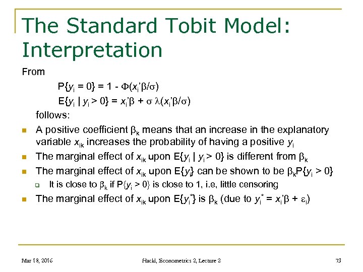The Standard Tobit Model: Interpretation From n n n P{yi = 0} = 1 - (xi’ / ) E{yi | yi > 0} = xi’ + (xi’ / ) follows: A positive coefficient k means that an increase in the explanatory variable xik increases the probability of having a positive yi The marginal effect of xik upon E{yi | yi > 0} is different from k The marginal effect of xik upon E{yi} can be shown to be k. P{yi > 0} q n It is close to k if P{yi > 0} is close to 1, i. e, little censoring The marginal effect of xik upon E{yi*} is k (due to yi* = xi’ + i) Mar 18, 2016 Hackl, Econometrics 2, Lecture 2 73

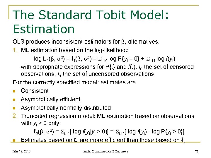The Standard Tobit Model: Estimation OLS produces inconsistent estimators for ; alternatives: 1. ML estimation based on the log-likelihood log L 1( , 2) = ℓ 1( , 2) = SiϵI 0 log P{yi = 0} + SiϵI 1 log f(yi) with appropriate expressions for P{. } and f(. ), I 0 the set of censored observations, I 1 the set of uncensored observations For the correctly specified model: estimates are n Consistent n Asymptotically efficient n Asymptotically normally distributed 2. Truncated regression model: ML estimation based on observations with yi > 0 only: ℓ 2( , 2) = SiϵI 1[ log f(yi|yi > 0)] = SiϵI 1[ log f(yi) - log P{yi > 0}] n Estimates based on ℓ 1 are more efficient than those based on ℓ 2 Mar 18, 2016 Hackl, Econometrics 2, Lecture 2 75

Example: Model for Budget Share for Tobacco and Alcohol Verbeek‘s data set TOBACCO: Belgian household budget survey of 1995/96; expenditures for tobacco and alcoholic beverages Budget share wi* for expenditures on alcoholic beverages corresponding to maximal utility: wi* = xi’ + I xi: log of total expenditures (LNX) and various characteristics like q q q number of children 2 years old (NKIDS 2) number of adults in household (NADULTS) Age (AGE) Actual budget share for expenditures on alcohol (SHARE 1, W 1) wi = wi* if wi* > 0, = 0 otherwise n 2724 households Mar 18, 2016 Hackl, Econometrics 2, Lecture 2 76

Model for Budget Share Budget share wi* for expenditures on alcoholic beverages wi* = xi’ + I regressors xi: q q q log of total expenditures (LNX) and household characteristics: AGE, NADULTS, NKIDS 2 interactions AGELNX (=LNX*AGE), NADLNX (=LNX*NADULTS) Actual budget share for expenditures on alcohol (SHARE 1, W 1) wi = wi* if wi* > 0, = 0 otherwise Attention! Sufficiently large change of income will create positive w* for any household! Mar 18, 2016 Hackl, Econometrics 2, Lecture 2 77

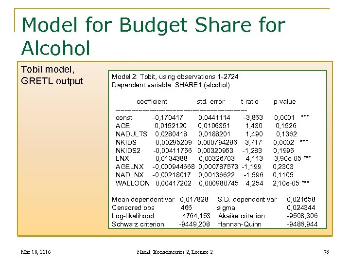Model for Budget Share for Alcohol Tobit model, GRETL output Model 2: Tobit, using observations 1 -2724 Dependent variable: SHARE 1 (alcohol) coefficient std. error t-ratio p-value ----------------------------- const -0, 170417 0, 0441114 -3, 863 0, 0001 *** AGE 0, 0152120 0, 0106351 1, 430 0, 1526 NADULTS 0, 0280418 0, 0188201 1, 490 0, 1362 NKIDS -0, 00295209 0, 000794286 -3, 717 0, 0002 *** NKIDS 2 -0, 00411756 0, 00320953 -1, 283 0, 1995 LNX 0, 0134388 0, 00326703 4, 113 3, 90 e-05 *** AGELNX -0, 000944668 0, 000787573 -1, 199 0, 2303 NADLNX -0, 00218017 0, 00136622 -1, 596 0, 1105 WALLOON 0, 00417202 0, 000980745 4, 254 2, 10 e-05 *** Mean dependent var 0, 017828 S. D. dependent var Censored obs 466 sigma Log-likelihood 4764, 153 Akaike criterion Schwarz criterion -9449, 208 Hannan-Quinn Mar 18, 2016 Hackl, Econometrics 2, Lecture 2 0, 021658 0, 024344 -9508, 306 -9486, 944 78

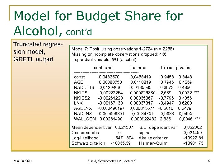Model for Budget Share for Alcohol, cont’d Truncated regression model, GRETL output Model 7: Tobit, using observations 1 -2724 (n = 2258) Missing or incomplete observations dropped: 466 Dependent variable: W 1 (alcohol) coefficient std. error t-ratio p-value ----------------------------- const 0, 0433570 0, 0458419 0, 9458 0, 3443 AGE 0, 00880553 0, 0110819 0, 7946 0, 4269 NADULTS -0, 0129409 0, 0185585 -0, 6973 0, 4856 NKIDS -0, 00222254 0, 000826380 -2, 689 0, 0072 *** NKIDS 2 -0, 00261220 0, 00335067 -0, 7796 0, 4356 LNX -0, 00167130 0, 00337817 -0, 4947 0, 6208 AGELNX -0, 000490197 0, 000815571 -0, 6010 0, 5478 NADLNX 0, 000806801 0, 00134731 0, 5988 0, 5493 WALLOON 0, 00261490 0, 000922432 2, 835 0, 0046 *** Mean dependent var 0, 021507 S. D. dependent var Censored obs 0 sigma Log-likelihood 5471, 304 Akaike criterion Schwarz criterion -10865, 39 Hannan-Quinn Mar 18, 2016 Hackl, Econometrics 2, Lecture 2 0, 022062 0, 021450 -10922, 61 -10901, 73 79

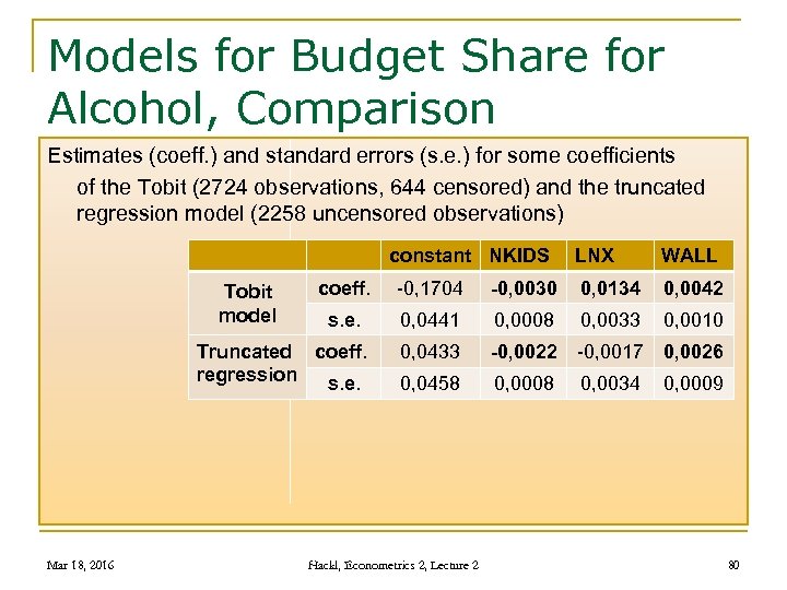Models for Budget Share for Alcohol, Comparison Estimates (coeff. ) and standard errors (s. e. ) for some coefficients of the Tobit (2724 observations, 644 censored) and the truncated regression model (2258 uncensored observations) constant NKIDS Tobit model WALL coeff. -0, 1704 -0, 0030 0, 0134 0, 0042 s. e. 0, 0441 0, 0008 0, 0033 0, 0010 0, 0433 -0, 0022 -0, 0017 0, 0026 0, 0458 0, 0008 0, 0034 0, 0009 Truncated coeff. regression s. e. Mar 18, 2016 LNX Hackl, Econometrics 2, Lecture 2 80

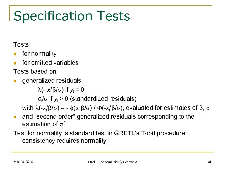Specification Tests n for normality n for omitted variables Tests based on n generalized residuals (- xi’ / ) if yi = 0 ei/ if yi > 0 (standardized residuals) with (-xi’ / ) = - (xi’ / ) / (-xi’ / ), evaluated for estimates of , n and “second order” generalized residuals corresponding to the estimation of 2 Test for normality is standard test in GRETL‘s Tobit procedure: consistency requires normality Mar 18, 2016 Hackl, Econometrics 2, Lecture 2 81

An Example: Modeling Wages Wage observations: available only for the working population Model that explains wages as a function of characteristics, e. g. , the person‘s age, gender, education, etc. n Low value of education increases probability of no wage q q n From a sample of wages the effect of education might be underestimated “Sample selection bias” Tobit model: for a positive coefficient of age, an increase of age q q q increases wage increases the probability that the person is working Not always realistic! Tobacco consumption: Abstention from smoking may be a person’s attitude not depending on factors which determine smoking intensity Mar 18, 2016 Hackl, Econometrics 2, Lecture 2 83

Modeling Wages, cont’d Tobit II model: allows two separate equations: n Equation for labor force participation of a person n Equation for the wage of a person Tobit II model is also called “sample selection model” Mar 18, 2016 Hackl, Econometrics 2, Lecture 2 84

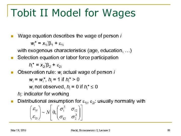Tobit II Model for Wages n n Wage equation describes the wage of person i wi* = x 1 i’ 1 + 1 i with exogenous characteristics (age, education, …) Selection equation or labor force participation hi* = x 2 i’ 2 + 2 i Observation rule: wi actual wage of person i wi = wi*, hi = 1 if hi* > 0 wi not observed, hi = 0 if hi* 0 hi: indicator for working Distributional assumption for 1 i, 2 i: usually normality with Mar 18, 2016 Hackl, Econometrics 2, Lecture 2 85

Model for Wages: Selection Equation Selection equation hi* = x 2 i’ 2 + 2 i: probit model for binary choice; standardization ( 22 = 1) n Characteristics x 1 i and x 2 i may be different; however, q q n If the selection depends upon wi*: x 2 i is expected to include x 1 i Because the model describes the joint distribution of wi and hi given one set of conditioning variables: x 2 i is expected to include x 1 i x 2 i should contain variables not included in x 1 i Sign and value of coefficients of the same variables in x 1 i and x 2 i are not the same Special cases q q If 12 = 0, sample selection is exogenous Tobit II model coincides with Tobit I model if x 1 i’ 1 = x 2 i’ 2 and 1 i = 2 i Mar 18, 2016 Hackl, Econometrics 2, Lecture 2 86

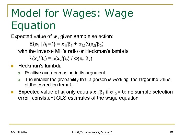Model for Wages: Wage Equation Expected value of wi, given sample selection: E{wi | hi =1} = x 1 i’ 1 + 12 (x 2 i’ 2) with the inverse Mill’s ratio or Heckman’s lambda (x 2 i’ 2) = (x 2 i’ 2) / (x 2 i’ 2) n Heckman’s lambda q q n Positive and decreasing in its argument The smaller the probability that a person is working, the larger the value of the correction term Expected value of wi only equals x 1 i’ 1 if 12 = 0: no sample selection error, consistent OLS estimates of the wage equation Mar 18, 2016 Hackl, Econometrics 2, Lecture 2 87

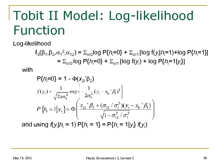Tobit II Model: Log-likelihood Function Log-likelihood ℓ 3( 1, 2, 12) = SiϵI 0 log P{hi=0} + SiϵI 1 [log f(yi|hi=1)+log P{hi=1}] = SiϵI 0 log P{hi=0} + SiϵI 1 [log f(yi) + log P{hi=1|yi}] with P{hi=0} = 1 - (x 2 i’ 2) and using f(yi|hi = 1) P{hi = 1} = P{hi = 1|yi} f(yi) Mar 18, 2016 Hackl, Econometrics 2, Lecture 2 88

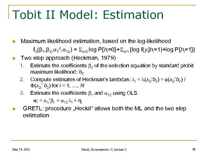Tobit II Model: Estimation n n Maximum likelihood estimation, based on the log-likelihood ℓ 3( 1, 2, 12) = SiϵI 0 log P{hi=0}+SiϵI 1 [log f(yi|hi=1)+log P{hi=1}] Two step approach (Heckman, 1979) 1. 2. 3. n Estimate the coefficients 2 of the selection equation by standard probit maximum likelihood: b 2 Compute estimates of Heckman’s lambdas: i = (x 2 i’b 2) / (x 2 i’ b 2) for i = 1, …, N Estimate the coefficients 1 and 12 using OLS wi = x 1 i’ 1 + 12 i + ηi GRETL: procedure „Heckit“ allows both the ML and the two step estimation Mar 18, 2016 Hackl, Econometrics 2, Lecture 2 89

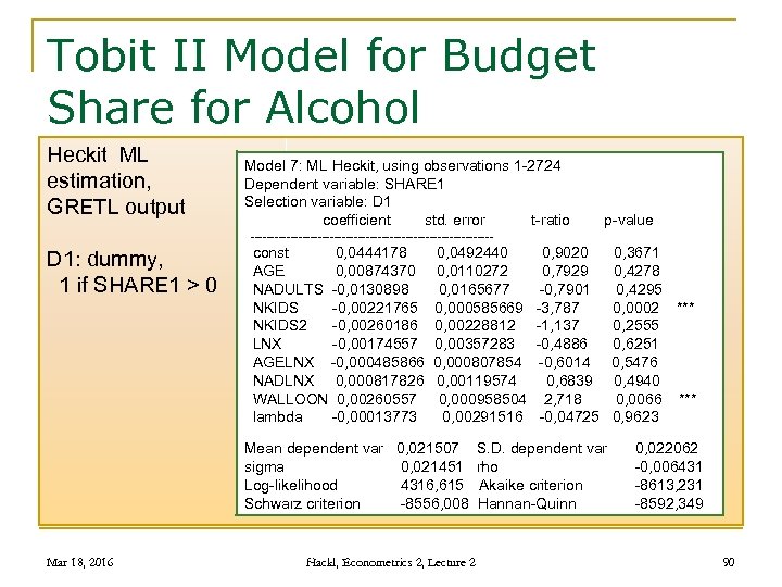Tobit II Model for Budget Share for Alcohol Heckit ML estimation, GRETL output Model 7: ML Heckit, using observations 1 -2724 Dependent variable: SHARE 1 Selection variable: D 1 coefficient std. error t-ratio p-value ------------------------------- D 1: dummy, 1 if SHARE 1 > 0 const 0, 0444178 0, 0492440 0, 9020 0, 3671 AGE 0, 00874370 0, 0110272 0, 7929 0, 4278 NADULTS -0, 0130898 0, 0165677 -0, 7901 0, 4295 NKIDS -0, 00221765 0, 000585669 -3, 787 0, 0002 *** NKIDS 2 -0, 00260186 0, 00228812 -1, 137 0, 2555 LNX -0, 00174557 0, 00357283 -0, 4886 0, 6251 AGELNX -0, 000485866 0, 000807854 -0, 6014 0, 5476 NADLNX 0, 000817826 0, 00119574 0, 6839 0, 4940 WALLOON 0, 00260557 0, 000958504 2, 718 0, 0066 *** lambda -0, 00013773 0, 00291516 -0, 04725 0, 9623 Mean dependent var 0, 021507 S. D. dependent var sigma 0, 021451 rho Log-likelihood 4316, 615 Akaike criterion Schwarz criterion -8556, 008 Hannan-Quinn Mar 18, 2016 Hackl, Econometrics 2, Lecture 2 0, 022062 -0, 006431 -8613, 231 -8592, 349 90

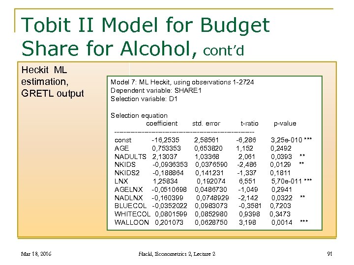Tobit II Model for Budget Share for Alcohol, cont’d Heckit ML estimation, GRETL output Model 7: ML Heckit, using observations 1 -2724 Dependent variable: SHARE 1 Selection variable: D 1 Selection equation coefficient std. error t-ratio p-value ------------------------------ const -16, 2535 2, 58561 -6, 286 3, 25 e-010 *** AGE 0, 753353 0, 653820 1, 152 0, 2492 NADULTS 2, 13037 1, 03368 2, 061 0, 0393 ** NKIDS -0, 0936353 0, 0376590 -2, 486 0, 0129 ** NKIDS 2 -0, 188864 0, 141231 -1, 337 0, 1811 LNX 1, 25834 0, 192074 6, 551 5, 70 e-011 *** AGELNX -0, 0510698 0, 0486730 -1, 049 0, 2941 NADLNX -0, 160399 0, 0748929 -2, 142 0, 0322 ** BLUECOL -0, 0352022 0, 0983073 -0, 3581 0, 7203 WHITECOL 0, 0801599 0, 0852980 0, 9398 0, 3473 WALLOON 0, 201073 0, 0628750 3, 198 0, 0014 *** Mar 18, 2016 Hackl, Econometrics 2, Lecture 2 91

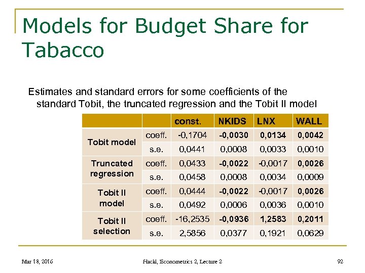Models for Budget Share for Tabacco Estimates and standard errors for some coefficients of the standard Tobit, the truncated regression and the Tobit II model const. NKIDS LNX WALL coeff. -0, 1704 -0, 0030 0, 0134 0, 0042 s. e. 0, 0441 0, 0008 0, 0033 0, 0010 Truncated regression coeff. 0, 0433 -0, 0022 -0, 0017 0, 0026 s. e. 0, 0458 0, 0008 0, 0034 0, 0009 Tobit II model coeff. 0, 0444 -0, 0022 -0, 0017 0, 0026 s. e. 0, 0492 0, 0006 0, 0036 0, 0010 -0, 0936 1, 2583 0, 2011 0, 0377 0, 1921 0, 0629 Tobit model Tobit II selection Mar 18, 2016 coeff. -16, 2535 s. e. 2, 5856 Hackl, Econometrics 2, Lecture 2 92

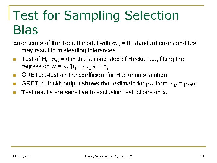Test for Sampling Selection Bias Error terms of the Tobit II model with 12 ≠ 0: standard errors and test may result in misleading inferences n Test of H 0: 12 = 0 in the second step of Heckit, i. e. , fitting the regression wi = x 1 i’ 1 + 12 i + ηi n GRETL: t-test on the coefficient for Heckman’s lambda n GRETL: Heckit-output shows rho, estimate for 12 from 12 = 12 1 n Test results are sensitive to exclusion restrictions on x 1 i Mar 18, 2016 Hackl, Econometrics 2, Lecture 2 93

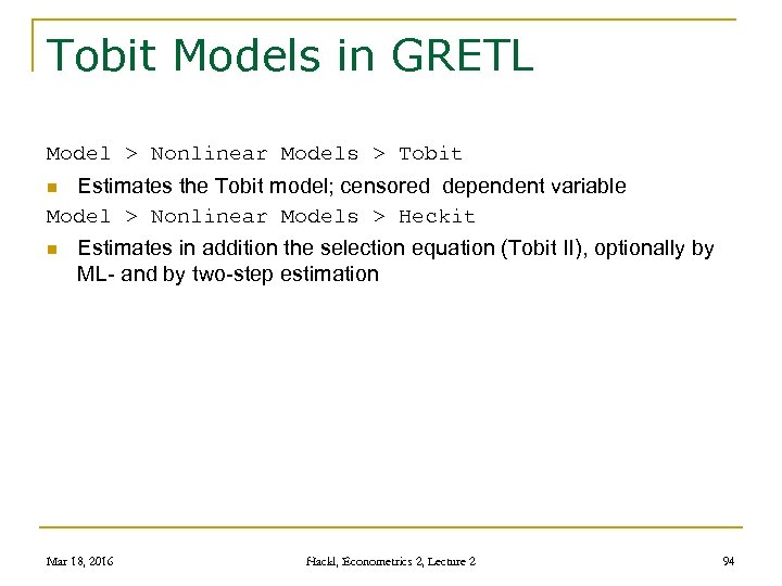Tobit Models in GRETL Model > Nonlinear Models > Tobit Estimates the Tobit model; censored dependent variable Model > Nonlinear Models > Heckit n n Estimates in addition the selection equation (Tobit II), optionally by ML- and by two-step estimation Mar 18, 2016 Hackl, Econometrics 2, Lecture 2 94

Your Homework 1. People buy for yi* assets of an investment fund, with yi* = xi’ + i, i ~ N(0, 2); xi consists of a “ 1” for the intercept and the variable income. The dummy di = 1 if yi* > 0 and di = 0 otherwise. a. Derive the probability for di = 1 as function of xi. b. Derive the log-likelihood function of the probit model for di, i = 1, . . . , N. c. Derive the ML estimator of the probability for di = 1 as function of xi of the logit model. 2. Verbeek‘s data set TOBACCO contains expenditures on tobacco in 2724 Belgian households, taken from the household budget survey of 1995/96, as well as other characteristics of the households; for the expenditures on tobacco, the dummy D 2=1 if the budget share for tobacco (SHARE 2) differs from 0, and D 2=0 otherwise. Mar 18, 2016 Hackl, Econometrics 2, Lecture 2 95

Your Homework, cont’d a. Model the budget share for tobacco, using (i) a Tobit model, (ii) a truncated regression, and (iii) a Tobit II model; using the household characteristics LNX, AGE, NKIDS, the interaction LNX*AGE, and the dummy FLANDERS; in addition BLUECOL for the selection equation. b. Compare the effects of the regressors in the three models, based on coefficients and t-statistics. c. Discuss the effect of the variable FLANDERS. Mar 18, 2016 Hackl, Econometrics 2, Lecture 2 96