Econ 616 Spring 2006 Qualitative Response Regression

Econ 616 – Spring 2006 Qualitative Response Regression Models Presented by Yan Hu 04/19/2006 Econ 616 1

Outline o Qualitative Response Regression Model o Binary Response Regression Models 1. 2. 3. The Linear Probability Model (LPM) The Logit Model The Probit Model 04/19/2006 Econ 616 2

What is Qualitative Response Regression Model? o The dependent variable is qualitative (or dummy) in nature. --- The dependent variable is a binary, or dichotomous variable: Y=1 if the person is in the labor force and Y=0 if he or she is not. --- Trichotomous response variable. --- Poly-chotomous (or multiplecategory) response variable. 04/19/2006 Econ 616 3

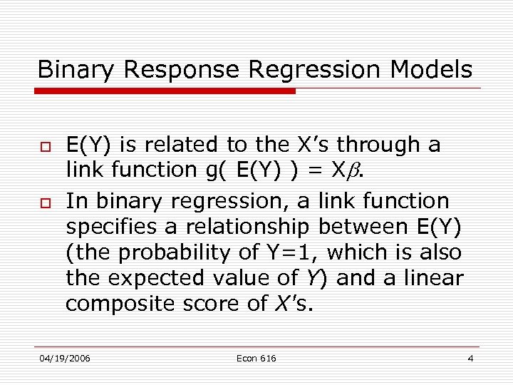Binary Response Regression Models o o E(Y) is related to the X’s through a link function g( E(Y) ) = X. In binary regression, a link function specifies a relationship between E(Y) (the probability of Y=1, which is also the expected value of Y) and a linear composite score of X's. 04/19/2006 Econ 616 4

Three Binary Response Regression Models o o o The Linear Probability Model (LPM) The Logit Model The Probit Model 04/19/2006 Econ 616 5

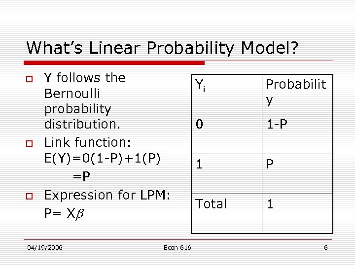What’s Linear Probability Model? o o o Y follows the Bernoulli probability distribution. Link function: E(Y)=0(1 -P)+1(P) =P Expression for LPM: P= X 04/19/2006 Econ 616 Yi Probabilit y 0 1 -P 1 P Total 1 6

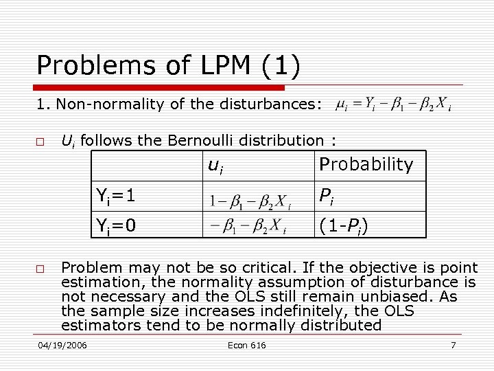Problems of LPM (1) 1. Non-normality of the disturbances: o Ui follows the Bernoulli distribution : ui Probability Yi=1 Yi=0 o Pi (1 -Pi) Problem may not be so critical. If the objective is point estimation, the normality assumption of disturbance is not necessary and the OLS still remain unbiased. As the sample size increases indefinitely, the OLS estimators tend to be normally distributed 04/19/2006 Econ 616 7

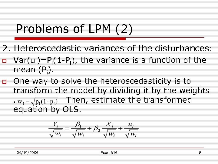Problems of LPM (2) 2. Heteroscedastic variances of the disturbances: o o Var(ui)=Pi(1 -Pi), the variance is a function of the mean (Pi). One way to solve the heteroscedasticity is to transform the model by dividing it by the weights. Then, estimate the transformed equation by OLS. 04/19/2006 Econ 616 8

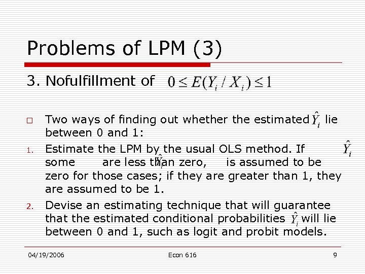Problems of LPM (3) 3. Nofulfillment of o 1. 2. Two ways of finding out whether the estimated lie between 0 and 1: Estimate the LPM by the usual OLS method. If some are less than zero, is assumed to be zero for those cases; if they are greater than 1, they are assumed to be 1. Devise an estimating technique that will guarantee that the estimated conditional probabilities will lie between 0 and 1, such as logit and probit models. 04/19/2006 Econ 616 9

Problems of LPM (4) 4. o o Questionable value of R 2 as a measure of goodness of fit. For a given X, the Y values will be either 0 or 1. Therefore, all the Y values will either lie along the Xaxis or along the line corresponding to 1. Therefore, generally no LPM is expected to fit such a scatter so well. As a result, the conventionally computed R 2 is likely to be much lower than 1 for such models. Aldrich and Nelson contend that “use of the coefficient of determination as a summary statistic shoud be avoided in models with qualitative dependent variable. ” 04/19/2006 Econ 616 10

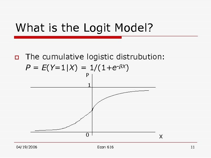What is the Logit Model? o The cumulative logistic distrubution: P = E(Y=1|X) = 1/(1+e-βX) P 1 0 04/19/2006 X Econ 616 11

What is the Logit Model? o o o From the logistic distribution, 1 -P = e-βX / (1+e-βX) P/(1 -P) = eβX, odds ratio log[p/(1 -P)] = βX Link function: g=log[ p/(1 -p) ], where p is the probability of either Y=1 or Y=0, depending on the software. Generally, log[ p/(1 -p) ]= X. 04/19/2006 Econ 616 12

Two Types of Data o To estimate the value of logit log[ p/(1 -p) ]= X, we have to distinguish two types of data: --- Data at the individual, or micro, level --- Grouped or replicated data 04/19/2006 Econ 616 13

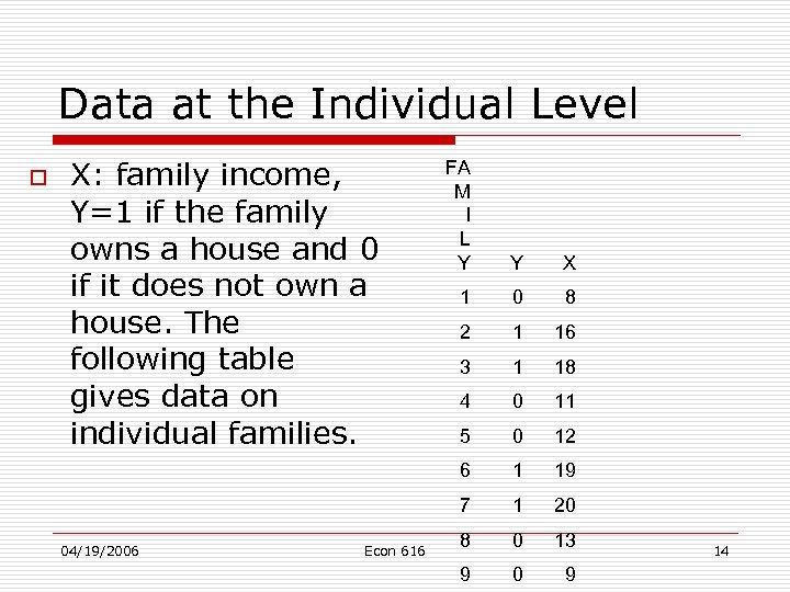Data at the Individual Level o X: family income, Y=1 if the family owns a house and 0 if it does not own a house. The following table gives data on individual families. X 1 0 8 2 1 16 3 1 18 4 0 11 5 0 12 1 19 7 Econ 616 Y 6 04/19/2006 FA M I L Y 1 20 8 0 13 9 0 9 14

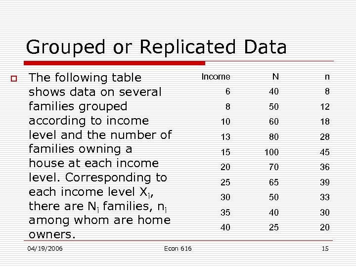Grouped or Replicated Data o The following table shows data on several families grouped according to income level and the number of families owning a house at each income level. Corresponding to each income level Xi, there are Ni families, ni among whom are home owners. 04/19/2006 Econ 616 Income N n 6 40 8 8 50 12 10 60 18 13 80 28 15 100 45 20 70 36 25 65 39 30 50 33 35 40 30 40 25 20 15

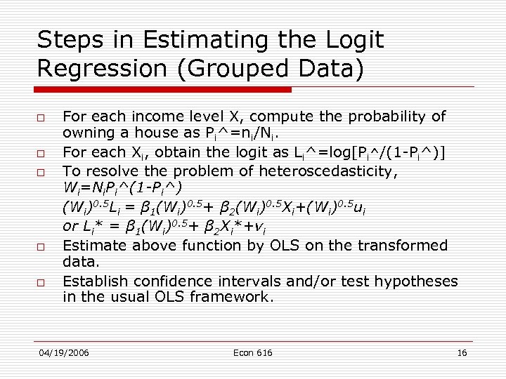Steps in Estimating the Logit Regression (Grouped Data) o o o For each income level X, compute the probability of owning a house as Pi^=ni/Ni. For each Xi, obtain the logit as Li^=log[Pi^/(1 -Pi^)] To resolve the problem of heteroscedasticity, Wi=Ni. Pi^(1 -Pi^) (Wi)0. 5 Li = β 1(Wi)0. 5+ β 2(Wi)0. 5 Xi+(Wi)0. 5 ui or Li* = β 1(Wi)0. 5+ β 2 Xi*+vi Estimate above function by OLS on the transformed data. Establish confidence intervals and/or test hypotheses in the usual OLS framework. 04/19/2006 Econ 616 16

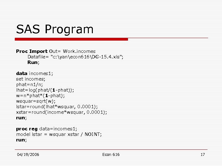SAS Program Proc Import Out= Work. incomes Datafile= "c: yanecon 616DG-15. 4. xls"; Run; data incomes 1; set incomes; phat=n 1/n; lhat=log(phat/(1 -phat)); w=n*phat*(1 -phat); wsquar=sqrt(w); lstar=round(lhat*wsquar, 0. 0001); xstar=round(income*wsquar, 0. 0001); run; proc reg data=incomes 1; model lstar = wsquar xstar / NOINT; run; 04/19/2006 Econ 616 17

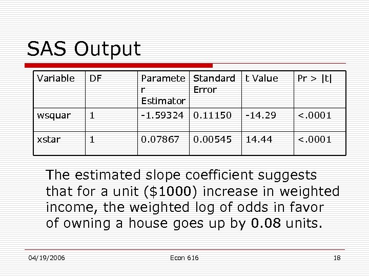SAS Output Variable DF Paramete Standard r Error Estimator t Value Pr > |t| wsquar 1 -1. 59324 0. 11150 -14. 29 <. 0001 xstar 1 0. 07867 0. 00545 14. 44 <. 0001 The estimated slope coefficient suggests that for a unit ($1000) increase in weighted income, the weighted log of odds in favor of owning a house goes up by 0. 08 units. 04/19/2006 Econ 616 18

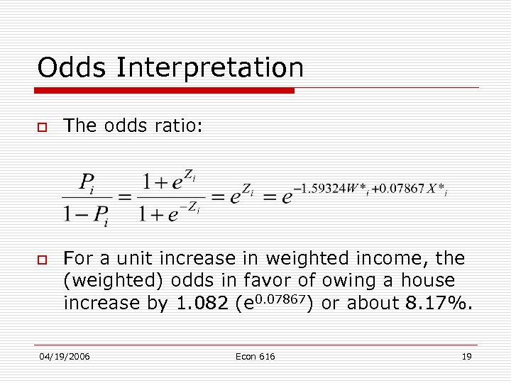Odds Interpretation o o The odds ratio: For a unit increase in weighted income, the (weighted) odds in favor of owing a house increase by 1. 082 (e 0. 07867) or about 8. 17%. 04/19/2006 Econ 616 19

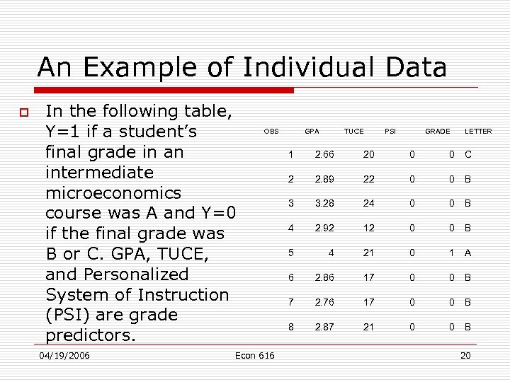An Example of Individual Data o In the following table, Y=1 if a student’s final grade in an intermediate microeconomics course was A and Y=0 if the final grade was B or C. GPA, TUCE, and Personalized System of Instruction (PSI) are grade predictors. 04/19/2006 OBS Econ 616 GPA TUCE PSI GRADE LETTER 1 2. 66 20 0 0 C 2 2. 89 22 0 0 B 3 3. 28 24 0 0 B 4 2. 92 12 0 0 B 5 4 21 0 1 A 6 2. 86 17 0 0 B 7 2. 76 17 0 0 B 8 2. 87 21 0 0 B 20

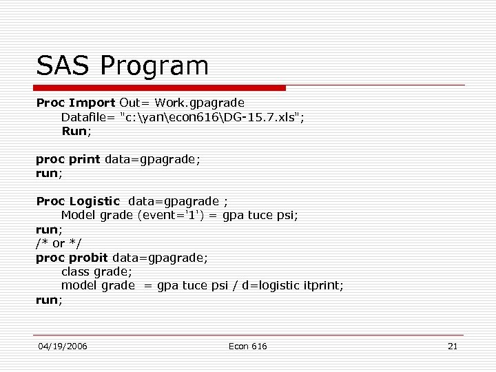SAS Program Proc Import Out= Work. gpagrade Datafile= "c: yanecon 616DG-15. 7. xls"; Run; proc print data=gpagrade; run; Proc Logistic data=gpagrade ; Model grade (event='1') = gpa tuce psi; run; /* or */ proc probit data=gpagrade; class grade; model grade = gpa tuce psi / d=logistic itprint; run; 04/19/2006 Econ 616 21

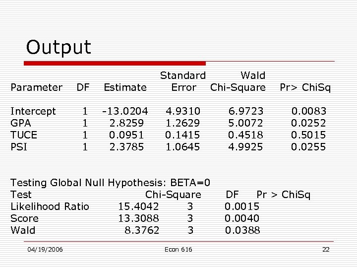Output Parameter Intercept GPA TUCE PSI DF Estimate 1 1 -13. 0204 2. 8259 0. 0951 2. 3785 Standard Wald Error Chi-Square 4. 9310 1. 2629 0. 1415 1. 0645 Testing Global Null Hypothesis: BETA=0 Test Chi-Square Likelihood Ratio 15. 4042 3 Score 13. 3088 3 Wald 8. 3762 3 04/19/2006 Econ 616 6. 9723 5. 0072 0. 4518 4. 9925 Pr> Chi. Sq 0. 0083 0. 0252 0. 5015 0. 0255 DF Pr > Chi. Sq 0. 0015 0. 0040 0. 0388 22

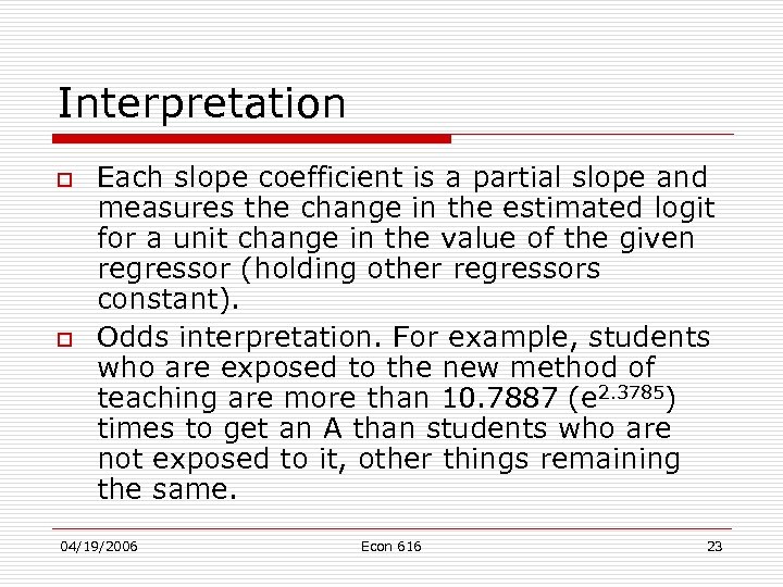Interpretation o o Each slope coefficient is a partial slope and measures the change in the estimated logit for a unit change in the value of the given regressor (holding other regressors constant). Odds interpretation. For example, students who are exposed to the new method of teaching are more than 10. 7887 (e 2. 3785) times to get an A than students who are not exposed to it, other things remaining the same. 04/19/2006 Econ 616 23

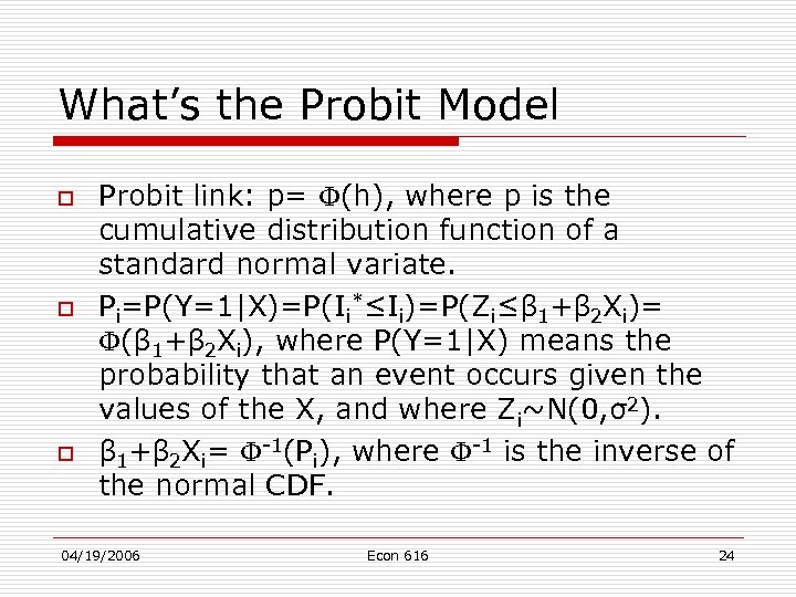What’s the Probit Model o o o Probit link: p= (h), where p is the cumulative distribution function of a standard normal variate. Pi=P(Y=1|X)=P(Ii*≤Ii)=P(Zi≤β 1+β 2 Xi)= (β 1+β 2 Xi), where P(Y=1|X) means the probability that an event occurs given the values of the X, and where Zi~N(0, σ2). β 1+β 2 Xi= -1(Pi), where -1 is the inverse of the normal CDF. 04/19/2006 Econ 616 24

Use of Probit Model o o Probit model is used when Y is considered as the “manifestation” of some unobservable Gaussian-distributed latent variable in the data. For example, the decision of the family to own a house or not depends on an unobservable index I (latent variable), that is determined by one or more explanatory variables, say income X, in such a way that the larger the value of the index I, the greater the probability of a family owning a house. 04/19/2006 Econ 616 25

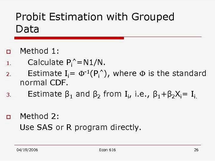Probit Estimation with Grouped Data o 1. 2. 3. o Method 1: Calculate Pi^=N 1/N. Estimate Ii= -1(Pi^), where is the standard normal CDF. Estimate β 1 and β 2 from Ii, i. e. , β 1+β 2 Xi= Ii. Method 2: Use SAS or R program directly. 04/19/2006 Econ 616 26

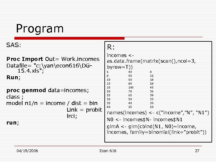Program SAS: Proc Import Out= Work. incomes Datafile= "c: yanecon 616DG 15. 4. xls"; Run; R: incomes

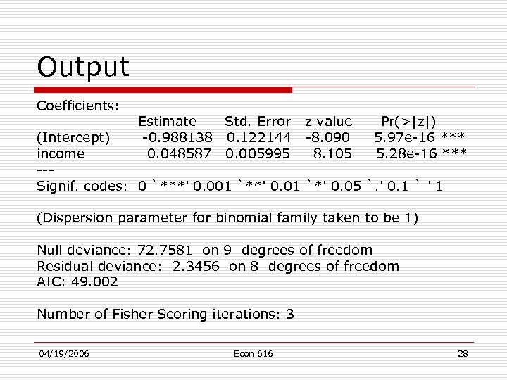Output Coefficients: Estimate Std. Error z value -0. 988138 0. 122144 -8. 090 0. 048587 0. 005995 8. 105 Pr(>|z|) 5. 97 e-16 *** 5. 28 e-16 *** (Intercept) income --Signif. codes: 0 `***' 0. 001 `**' 0. 01 `*' 0. 05 `. ' 0. 1 ` ' 1 (Dispersion parameter for binomial family taken to be 1) Null deviance: 72. 7581 on 9 degrees of freedom Residual deviance: 2. 3456 on 8 degrees of freedom AIC: 49. 002 Number of Fisher Scoring iterations: 3 04/19/2006 Econ 616 28

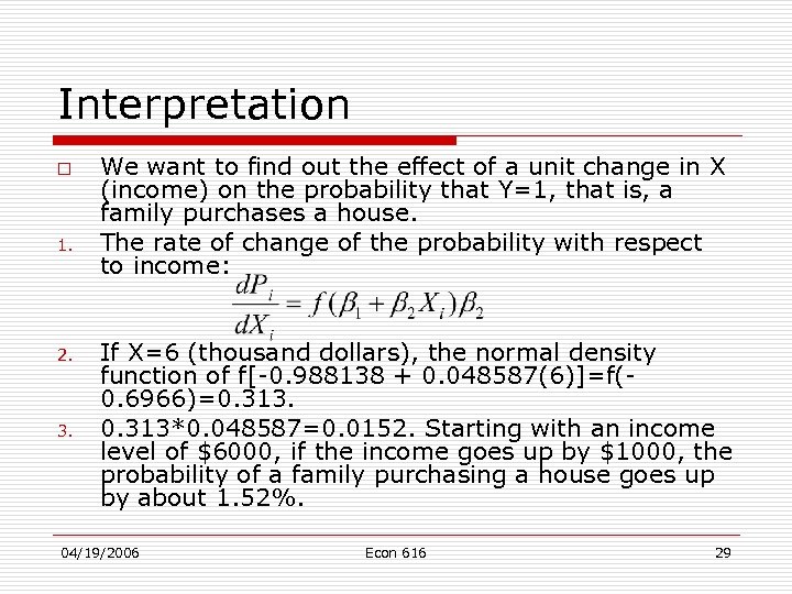Interpretation o 1. 2. 3. We want to find out the effect of a unit change in X (income) on the probability that Y=1, that is, a family purchases a house. The rate of change of the probability with respect to income: If X=6 (thousand dollars), the normal density function of f[-0. 988138 + 0. 048587(6)]=f(0. 6966)=0. 313*0. 048587=0. 0152. Starting with an income level of $6000, if the income goes up by $1000, the probability of a family purchasing a house goes up by about 1. 52%. 04/19/2006 Econ 616 29

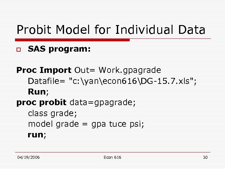Probit Model for Individual Data o SAS program: Proc Import Out= Work. gpagrade Datafile= "c: yanecon 616DG-15. 7. xls"; Run; proc probit data=gpagrade; class grade; model grade = gpa tuce psi; run; 04/19/2006 Econ 616 30

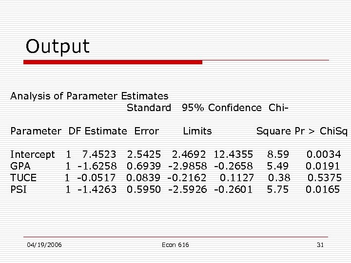Output Analysis of Parameter Estimates Standard 95% Confidence Chi- Parameter DF Estimate Error Limits Intercept 1 7. 4523 2. 5425 2. 4692 12. 4355 GPA 1 -1. 6258 0. 6939 -2. 9858 -0. 2658 TUCE 1 -0. 0517 0. 0839 -0. 2162 0. 1127 PSI 1 -1. 4263 0. 5950 -2. 5926 -0. 2601 04/19/2006 Econ 616 Square Pr > Chi. Sq 8. 59 5. 49 0. 38 5. 75 0. 0034 0. 0191 0. 5375 0. 0165 31

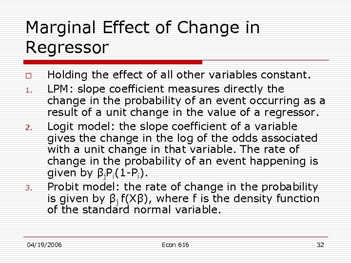Marginal Effect of Change in Regressor o 1. 2. 3. Holding the effect of all other variables constant. LPM: slope coefficient measures directly the change in the probability of an event occurring as a result of a unit change in the value of a regressor. Logit model: the slope coefficient of a variable gives the change in the log of the odds associated with a unit change in that variable. The rate of change in the probability of an event happening is given by βj. Pi(1 -Pi). Probit model: the rate of change in the probability is given by βj f(Xβ), where f is the density function of the standard normal variable. 04/19/2006 Econ 616 32

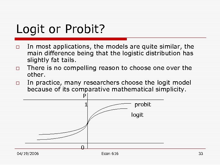Logit or Probit? o o o In most applications, the models are quite similar, the main difference being that the logistic distribution has slightly fat tails. There is no compelling reason to choose one over the other. In practice, many researchers choose the logit model because of its comparative mathematical simplicity. P 1 probit logit 0 04/19/2006 Econ 616 33

Reading o Damodar N. Gujarati, Basic Econometrics, P 580 -615 04/19/2006 Econ 616 34