ECON 454 INCIDENCE OF TAXATION AND THE EXCESS

ECON 454 INCIDENCE OF TAXATION AND THE EXCESS BURDEN (WELFARE COST) OF TAXATION E. Nketiah-Amponsah Department of Economics enamponsah@ug. edu. gh 1

Introduction Many policies centre around whether the tax burden is distributed fairly. Who then bears the final burden (cost) of a tax? The study of tax incidence attempts to determine who in the economy bears the final “burden” of taxation. Taxes affect relative prices, causing changes in resource allocation and prices. It is possible that the party which is legally responsible for the tax may not necessarily be the one who bears the burden of the tax. Tax incidence is the division/distribution of the burden of a tax between the buyer and the seller. Statutory/Legal incidence/Formal: Who is statutorily or legally responsible for the tax. Economic /Effective Incidence: The true change in the distribution of income induced by the tax. That is who bears the real or final burden of the tax. These two concepts differ because of tax shifting. But what really matters is the economic incidence of the tax. 2

Introduction Tax incidence: the difference between the prices paid/received and the price in the absence of the tax The distribution of the tax burden between the consumer and the producer The less flexible party pays the larger burden. Inelasticity is expensive 3

Introd-Cont The parties on whom the tax is imposed may not be the parties who actually or ultimately pay it A firm must statutorily pay a tax but the economic incidence may be shifted to other people such as the consumer via higher prices (i. e. forward shift) A firm may shift part of the tax burden onto factor owners (backward shift) All taxes formally incident on businesses will have their final incidence on customers, shareholders and employees: • Sales Taxes – Are Passed on and affect prices and customers, also 4 output and employees. • Profits Tax – Affect shareholders and investment decisions (suppliers of capital). • Asset Taxes – Affect investment decisions.

Introd-Cont For e. g. , if a wage tax is imposed and the supply of labour falls, the market clearing wage rate would rise and this would increase the cost of labour to producers. The impact of the wage tax and, hence, the incidence of the wage tax would be on workers as well as employers. 5

Partial Equilibrium Analysis of Tax incidence Partial equilibrium models only examine the market in which the tax is imposed, and ignores other markets Most appropriate when the taxed commodity is small relative to the economy as a whole. • Tax incidence depends on the elasticities of demand supply. In general, the more elastic the demand curve, the less of the tax is borne by consumers, ceteris paribus. Elasticity provides a measure of an economy agent’s ability to ‘escape’ the tax The more elastic the demand, the easier it is for consumers to turn to other products when the price goes up (i. e. suppliers must bear more of the tax) Incidence also depends on how prices are determined Industry structure matters Short-run vs. long run responses. 6

Partial Equilibrium Analysis of Tax incidence Graphically, there are three ways to determine the tax’s effect (burden): Shift the supply curve up by T Shift the demand curve down by T Use a wedge between the amounts consumers pay and firms receive All three methods yield the same results Makes no difference whether the tax is levied on consumers or producers 7

We’ll consider the Imposition of; Per Unit Tax: A tax that is specified as a fixed amount for each unit of a good sold. Ex. excise taxes on gasoline and cigarettes fall into this per unit tax category. Ex GHS 2 per pack of cigarette, per gallon of petrol, per litre of alcohol etc Excise Tax: A tax on the manufacture or sale of a particular (selected) good or service such as petroleum, tobacco and alcoholic beverages. Lump sum tax is a tax that must be paid regardless of the taxpayer’s behavior(income). 8 Ad valorem a percentage of the value of the goods or services sold. For. Ex. 17. 5%, 20% of the value of the product

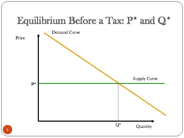Equilibrium Before a Tax: P* and Q* Demand Curve Price Supply Curve P* Q* 9 Quantity

Now Introduce a Tax Demand Curve Price Supply Curve including tax P** Tax Supply Curve P* 10 Q** Q* Quantity

Some Obvious Consequences 1. Consumers are paying more for each unit. (bad) 2. Government is earning taxes. (might be good) 3. Consumers are buying fewer units. (bad) 4. Firms are making fewer units. (Neutral here as perfect competition implies they make zero profit) 5. In studying the effects of taxes it’s important to distinguish between the amount a consumer pays for a good and the amount a firm receives 11 Wedge created by the tax

Tax Revenue = Tax per unit multiplied by the Number of Units sold Demand Curve Price Supply Curve including tax P** Tax Revenue Supply Curve P* 12 Q** Q* Quantity

Tax Revenue = Exactly the losses of consumers who still buy Demand Curve Price Supply Curve including tax P** Extra Paid by Consumers Supply Curve P* 13 Q** Q* Quantity

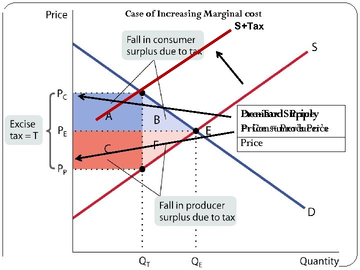Case of Increasing Marginal cost S+Tax Pre-Tax Supply Demand Price = Producer’s = Consumer’s Price 14

The Substitution Effect The price of this commodity has risen relative to other commodities. This affects the incentive of the private sector. It distorts markets. Notice that – less goods are produced. Some consumers don’t buy at the higher price. Some sellers don’t produce at the lower price. It generates “rents” A tax on tobacco for example, makes growing it less attractive, therefore land prices fall. Tobacco machinery manufacturers lose as do tobacco workers. 15 (Any input into a taxed commodity suffers. )

Shifting the Demand Curve 16 15 -16

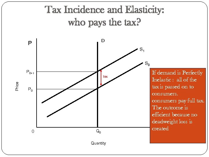Tax Incidence and Elasticity: who pays the tax? D P S 1 S 0 Price P 0+ t tax P 0 0 Quantity If demand is Perfectly Inelastic : all of the tax is passed on to consumers pay full tax. The outcome is efficient because no deadweight loss is created Q

Price per gallon (P) D S 2 S 1 P 2 = $2. 00 With perfectly inelastic demand, consumers bear the full burden. Consumer burden P 1 = $1. 50 $0. 50 Q 1 = 100 18 Quantity in billions of gallons (Q)

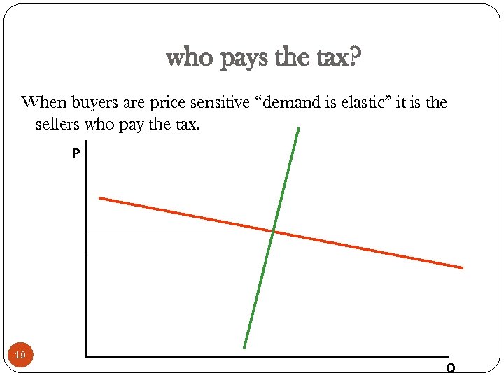who pays the tax? When buyers are price sensitive “demand is elastic” it is the sellers who pay the tax. P 19 Q

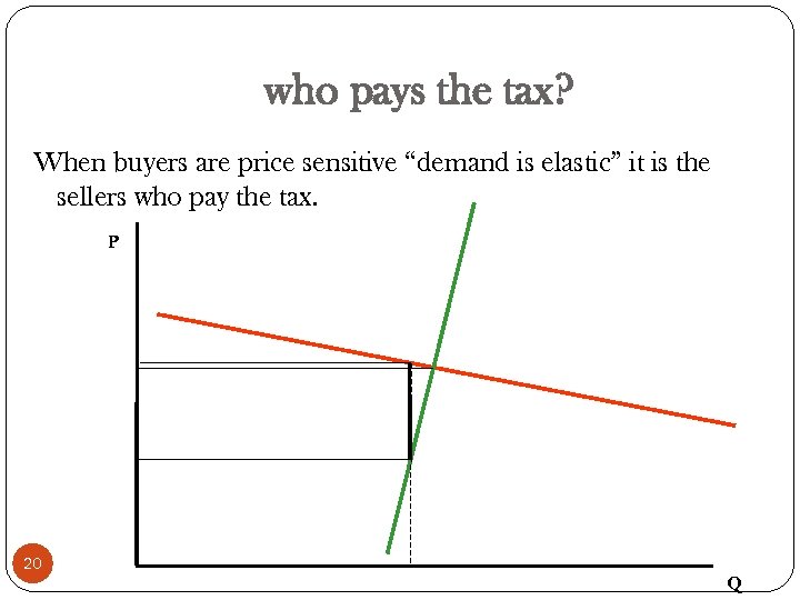who pays the tax? When buyers are price sensitive “demand is elastic” it is the sellers who pay the tax. P 20 Q

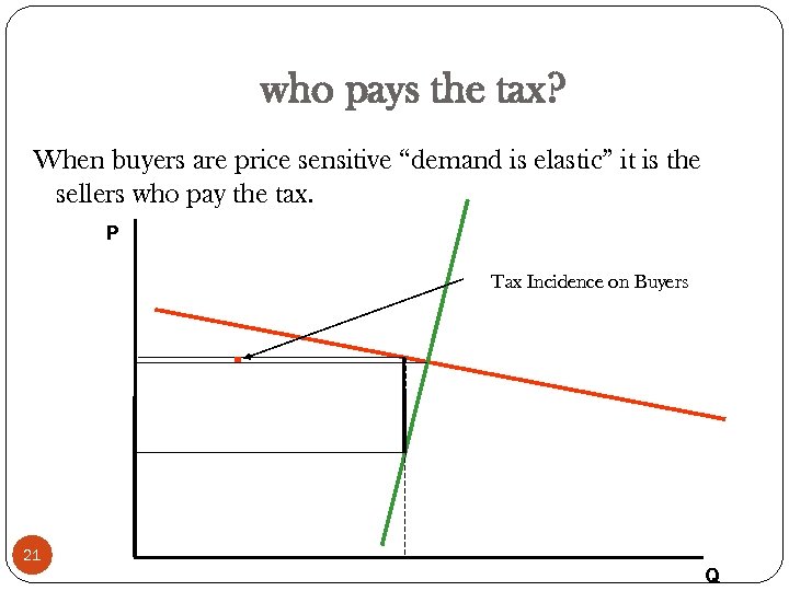who pays the tax? When buyers are price sensitive “demand is elastic” it is the sellers who pay the tax. P Tax Incidence on Buyers 21 Q

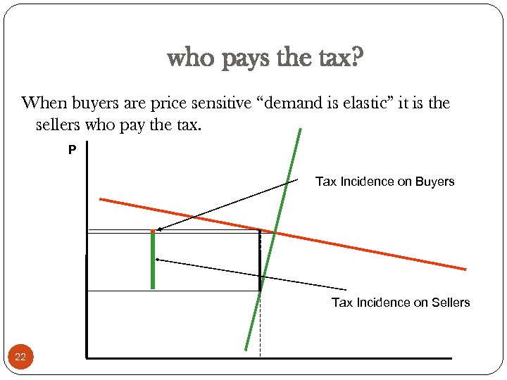who pays the tax? When buyers are price sensitive “demand is elastic” it is the sellers who pay the tax. P Tax Incidence on Buyers Tax Incidence on Sellers 22

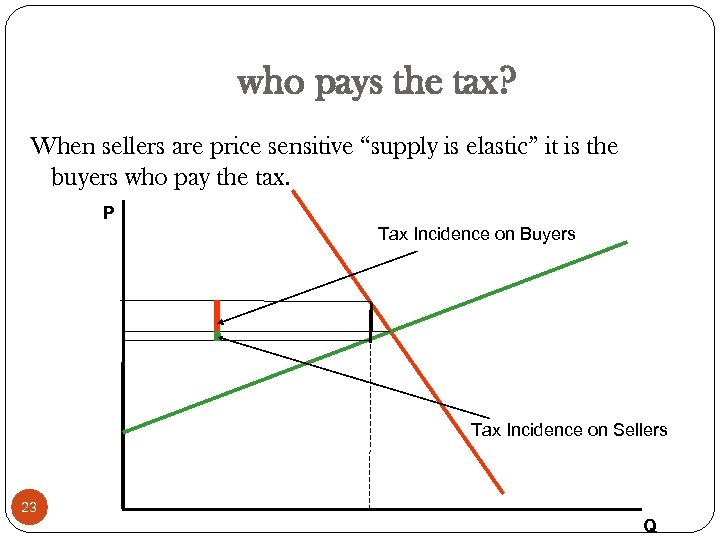who pays the tax? When sellers are price sensitive “supply is elastic” it is the buyers who pay the tax. P Tax Incidence on Buyers Tax Incidence on Sellers 23 Q

Who pays the tax? Demand Curve Price When seller/producers are completely price-sensitive, consumers pay the tax Supply Curve including tax P** Tax Revenue Supply Curve P* 24 Q** Q* Quantity

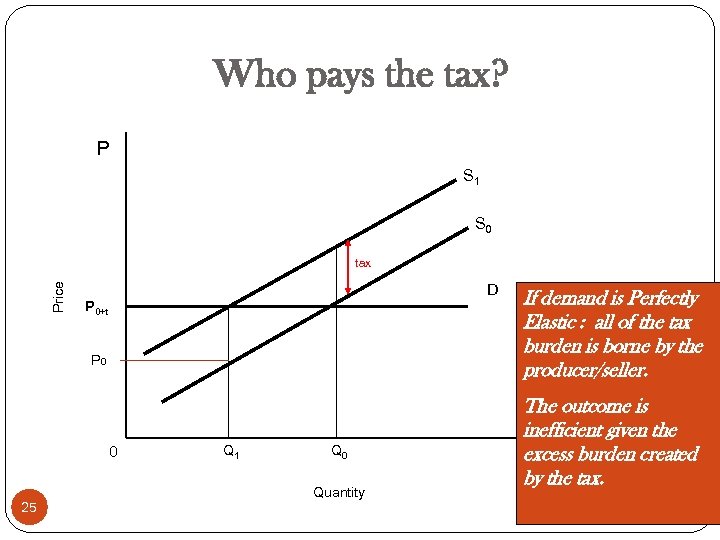Who pays the tax? P S 1 S 0 Price tax D P 0+t P 0 0 25 Q 1 Q 0 Quantity If demand is Perfectly Elastic : all of the tax burden is borne by the producer/seller. The outcome is inefficient given the Q excess burden created by the tax.

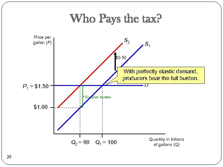Who Pays the tax? Price per gallon (P) S 2 S 1 $0. 50 With perfectly elastic demand, producers bear the full burden. D P 1 = $1. 50 Supplier burden $1. 00 Q 2 = 90 26 Q 1 = 100 Quantity in billions of gallons (Q)

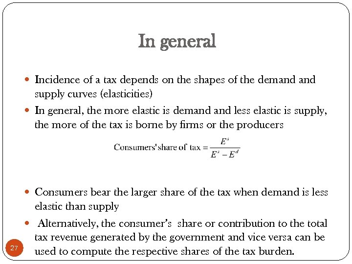In general Incidence of a tax depends on the shapes of the demand supply curves (elasticities) In general, the more elastic is demand less elastic is supply, the more of the tax is borne by firms or the producers Consumers bear the larger share of the tax when demand is less 27 elastic than supply Alternatively, the consumer’s share or contribution to the total tax revenue generated by the government and vice versa can be used to compute the respective shares of the tax burden.

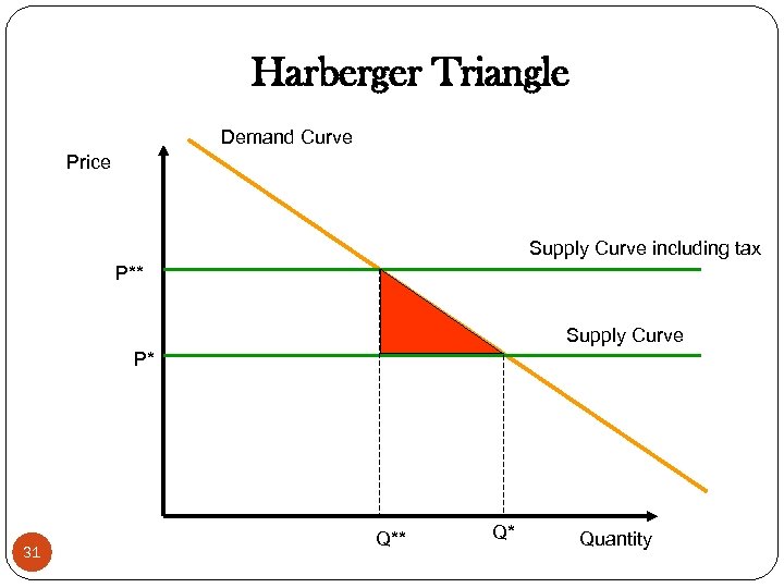
Excess Burden Excess burden is a loss of welfare above and beyond the tax revenues collected. It is the magnitude of the economic costs accompanying economic distortions (Hines, 2007) Also known as deadweight loss and welfare cost of taxation A tax causes a deadweight loss to society, because less of the good is produced and consumed than in the absence of the tax. Excess burden could be measured using demand curves. EB however, depends on substitution effect of the price change brought about by the tax. Thus a compensated response (a movement along the same indifference curve) is the important consideration when discussing excess burden. 28

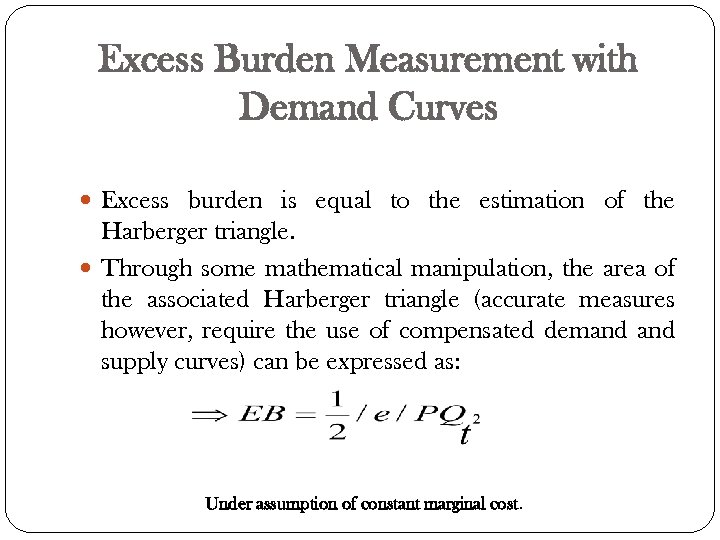Excess Burden Measurement with Demand Curves Excess burden is equal to the estimation of the Harberger triangle. Through some mathematical manipulation, the area of the associated Harberger triangle (accurate measures however, require the use of compensated demand supply curves) can be expressed as: 29 Under assumption of constant marginal cost.

Excess Burden Measurement with Demand Curves Implications of formula: Higher (compensated) elasticities lead to larger excess burden. Excess burden increases with the square of the tax rate. The greater the initial expenditure on the taxed commodity, the larger the excess burden. A good tax system should impose taxes with least excess burden first. Then move on to those taxes with higher excess burden. Optimally, the marginal excess burden of each tax 30 instrument should be the same.

Harberger Triangle Demand Curve Price Supply Curve including tax P** Supply Curve P* 31 Q** Q* Quantity

EB With Increasing Marginal Cost In general, the supply curve is upward sloping rather (increasing marginal cost) than horizontal. Welfare cost of lump-sum tax under increasing marginal cost See diagram in the next slide 32

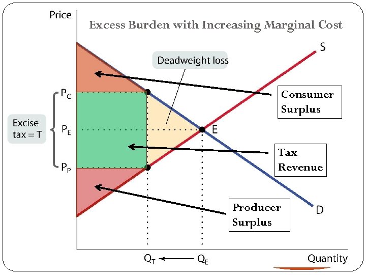Excess Burden with Increasing Marginal Cost Consumer Surplus Tax Revenue Producer Surplus 33

Subsidy and Excess Burden Subsidies as well as taxes create excess burden 34

EB With Ad Valorem Tax An ad-valorem tax is a tax with a rate given in price. proportion to the A good example is the sales tax (VAT). Graphical analysis is fairly similar to the case we had with the per unit tax Instead of moving the demand curve down by the same absolute amount for each quantity, move it down by the same proportion. Consider a case of an ad-valorem tax levied on demanders. As with the per-unit tax, the demand curve as perceived by suppliers has changed, and the same analysis is used to find equilibrium quantity and prices. 35

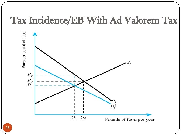Tax Incidence/EB With Ad Valorem Tax 36

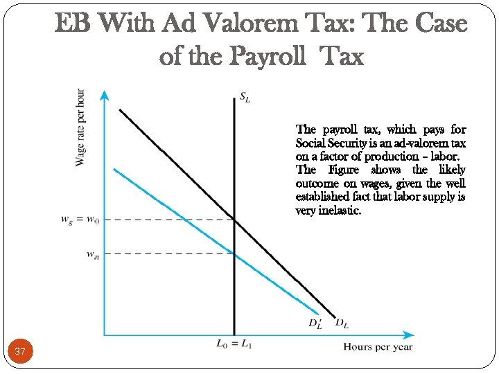EB With Ad Valorem Tax: The Case of the Payroll Tax The payroll tax, which pays for Social Security is an ad-valorem tax on a factor of production – labor. The Figure shows the likely outcome on wages, given the well established fact that labor supply is very inelastic. 37

Elasticity and Deadweight Loss General rule for economic policy: Other things equal, you want to choose the policy that produces the smallest deadweight loss. But how can we predict the size of the deadweight loss associated with a given policy? When demand, supply, or both, is inelastic it will cause a relatively smaller deadweight loss. 38

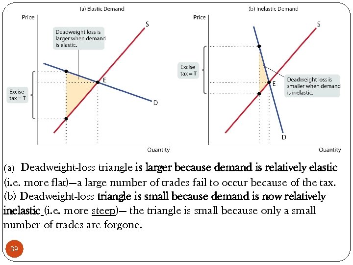(a) Deadweight-loss triangle is larger because demand is relatively elastic (i. e. more flat)—a large number of trades fail to occur because of the tax. (b) Deadweight-loss triangle is small because demand is now relatively inelastic (i. e. more steep)— the triangle is small because only a small number of trades are forgone. 39

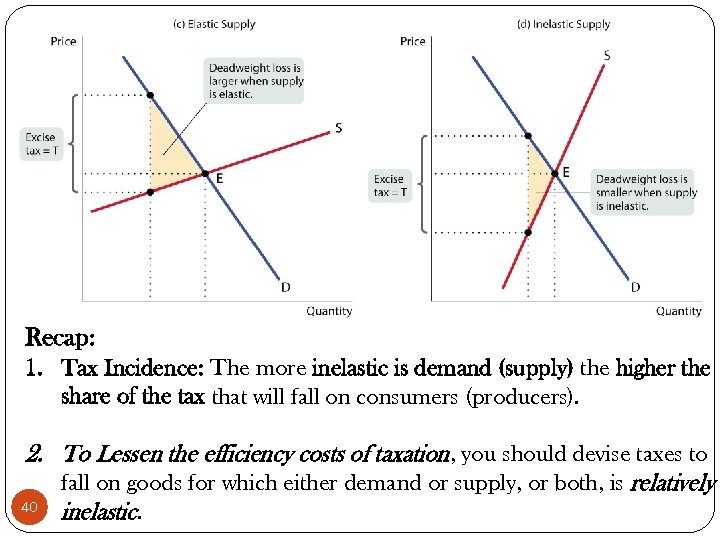Recap: 1. Tax Incidence: The more inelastic is demand (supply) the higher the share of the tax that will fall on consumers (producers). 2. To Lessen the efficiency costs of taxation, you should devise taxes to fall on goods for which either demand or supply, or both, is relatively 40 inelastic.

Taxes and Market Structure • The imposition of a lump sum tax (T) or equivalently a percentage of a profit tax ) and a specific excise tax (t) constant per unit of output could be considered under conditions of perfect competition and monopoly. • Now let’s relax the assumption of perfect competition. • The figure below shows a monopolist before a per-unit tax is imposed • The key to analyzing the effects of these two type of taxes is isolating the way in which cost curves are effected by taxes. 41

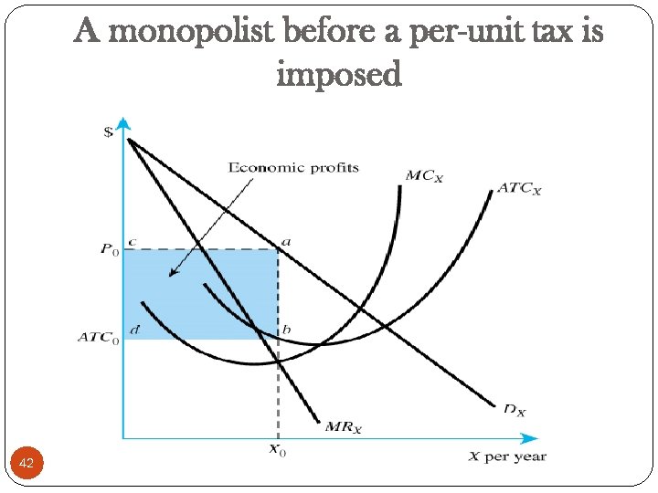A monopolist before a per-unit tax is imposed 42

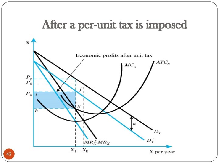After a per-unit tax is imposed 43

Monopolist Profit Falls o After a per-unit tax is imposed (as in above), the “effective” demand curve shifts down, as does the “effective” marginal revenue curve. o Monopolist’s profits fall after the tax, even though it has market power. o Firms can be taxed on economic profits, defined as the return to the owners of the firm in excess of the opportunity costs of the factors used in production. 44

Efficiency Loss Ratio of a Tax To compare the relative loss in efficiency of various taxes, economist often compute the excess burden per cedi or dollar of tax revenue. The ratio of the excess burden of a tax to the tax revenue collected each year by that tax is referred to as the efficiency-loss ratio. An efficiency loss ratio of 0. 25 means that the excess burden of a tax is 25 pesewas for each cedi of revenue raised per specified time period (per month, annum) 45

General Equilibrium Thus far, we have limited our analysis to only the impact of taxes on a single market. In the real world, a system of taxes affects many markets and results in resource flows among many sectors of the economy. General or multi-market analysis of excess burden is important in getting a realistic picture of the impact of taxes on resource use. Provides insight to help us reduce the efficiency loss from taxes Given the complex interrelated nature of markets, the effect of a tax in any one market affects related markets with possible feedback effects in the market initially taxed. For example, a tax on the consumption of electric power, in addition to affecting the price of electricity, affects the demand for various electrical appliances, and for natural gas for coking and heating. The shifts in demand affects the prices of those substitutes and complements. 46

General Equilibrium-Cont For instance, a flat rate sales tax of t percent on both food and clothing results in greater excess burden in the clothing market than in the food market. Why? Diagram Total excess burden can be reduced by increasing the tax rate on food and lowering the tax rate on clothing until the marginal increase in the excess burden in the food market equals the marginal decrease in the excess burden in the clothing market. A tax on output in one market can affect prices in other markets. A tax-induced increase in the price of clothing, causes inputs to flow into the food industry. This increases the supply of food and decreases its price. 47

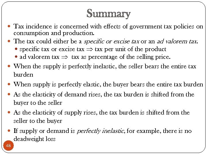Summary Tax incidence is concerned with effects of government tax policies on 48 consumption and production. The tax could either be a specific or excise tax or an ad valorem tax. specific tax or excise tax per unit of the product ad valorem tax as percentage of the selling price. When the supply is perfectly inelastic, the seller bears the entire tax burden When supply is perfectly elastic, the buyer bears the entire tax burden As the elasticity of demand rises, the tax burden is shifted from the buyer to the seller As the elasticity of supply rises, the tax burden is shifted from the seller to the buyer If supply or demand is perfectly inelastic, for example, there is no deadweight loss

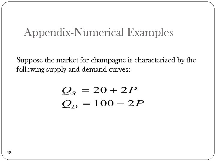Appendix-Numerical Examples Suppose the market for champagne is characterized by the following supply and demand curves: 49

Appendix-Numerical Examples If the government imposes a per-unit tax on demanders of $8 per unit, the tax creates a wedge between what demanders pay and suppliers get. Before the tax, we can rewrite the system as: 50

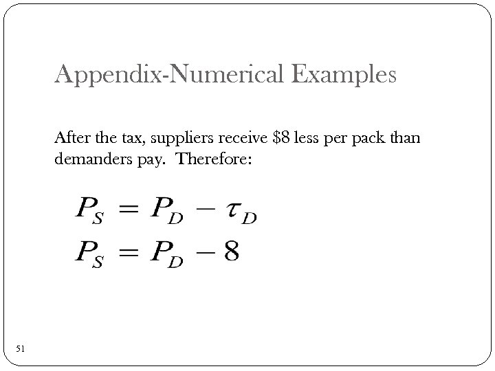Appendix-Numerical Examples After the tax, suppliers receive $8 less per pack than demanders pay. Therefore: 51

Appendix-Numerical Examples Solving the initial system (before the tax) gives a price of P=20 and Q=60. Solving the system after the tax gives: 52

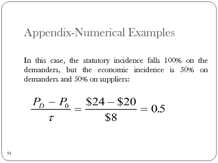Appendix-Numerical Examples In this case, the statutory incidence falls 100% on the demanders, but the economic incidence is 50% on demanders and 50% on suppliers: 53

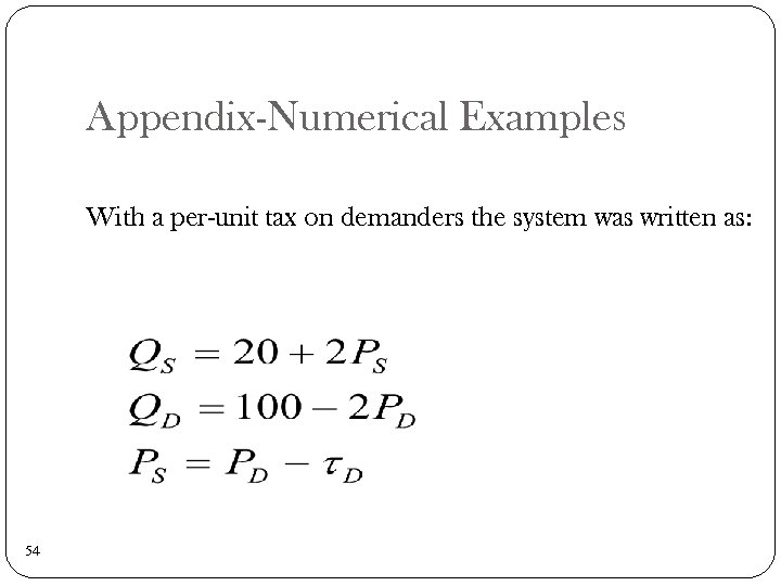Appendix-Numerical Examples With a per-unit tax on demanders the system was written as: 54

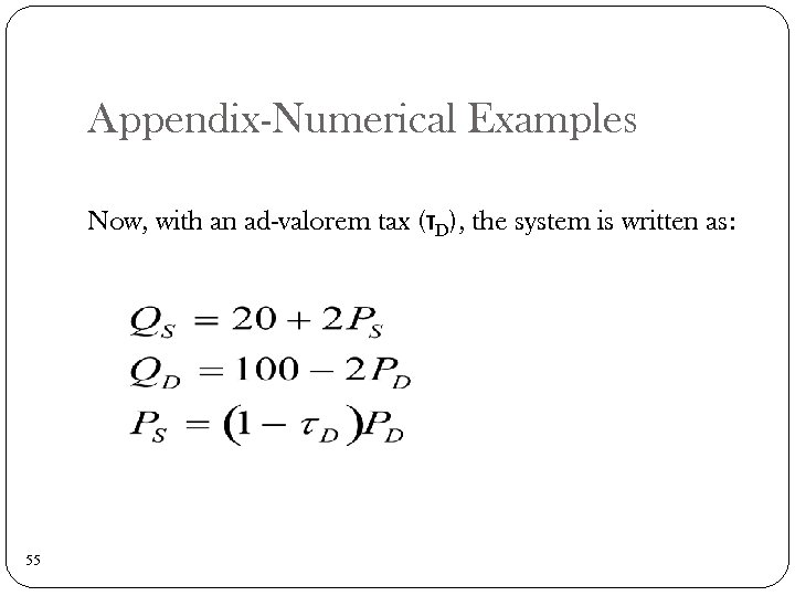Appendix-Numerical Examples Now, with an ad-valorem tax (τD), the system is written as: 55

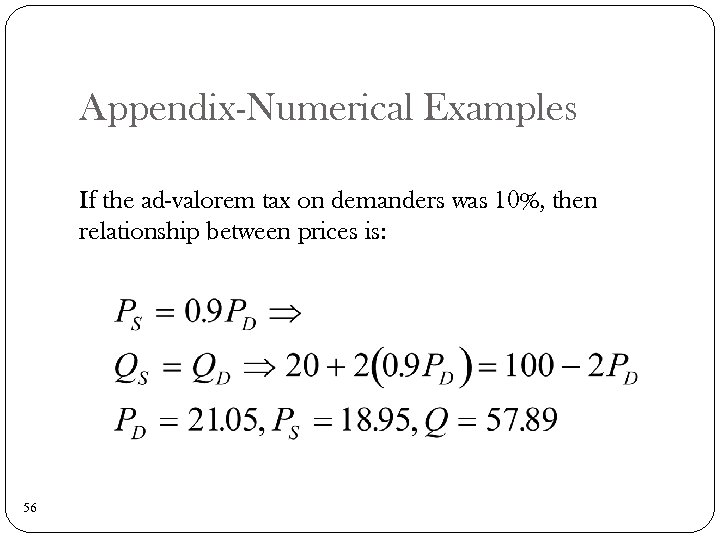Appendix-Numerical Examples If the ad-valorem tax on demanders was 10%, then relationship between prices is: 56

Further Exercises Also see accompanying trial exercises 57