b60b4209313f42572da6268bad3da236.ppt
- Количество слайдов: 25
Econ 140 Bivariate Populations Lecture 5 1
Today’s Plan Econ 140 • Bivariate populations and conditional probabilities • Joint and marginal probabilities • Bayes Theorem Lecture 5 2
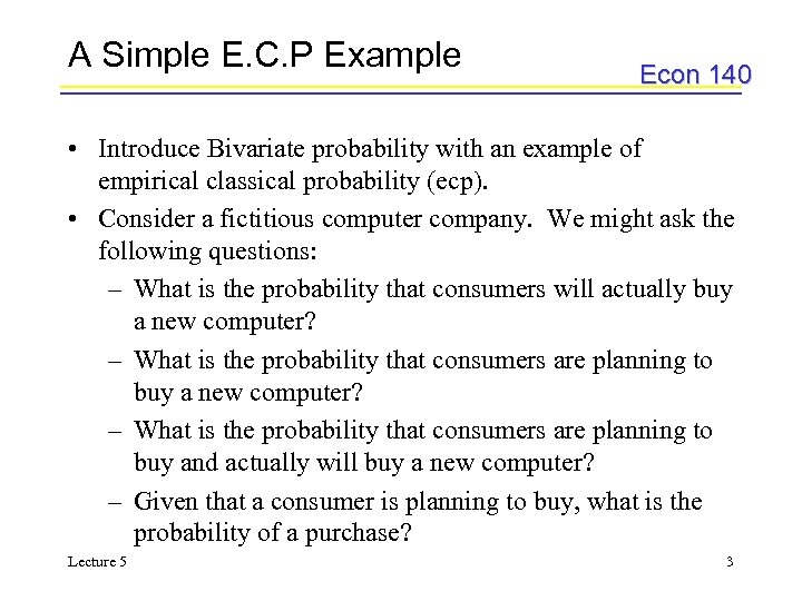
A Simple E. C. P Example Econ 140 • Introduce Bivariate probability with an example of empirical classical probability (ecp). • Consider a fictitious computer company. We might ask the following questions: – What is the probability that consumers will actually buy a new computer? – What is the probability that consumers are planning to buy and actually will buy a new computer? – Given that a consumer is planning to buy, what is the probability of a purchase? Lecture 5 3
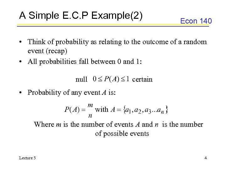
A Simple E. C. P Example(2) Econ 140 • Think of probability as relating to the outcome of a random event (recap) • All probabilities fall between 0 and 1: null certain • Probability of any event A is: Where m is the number of events A and n is the number of possible events Lecture 5 4
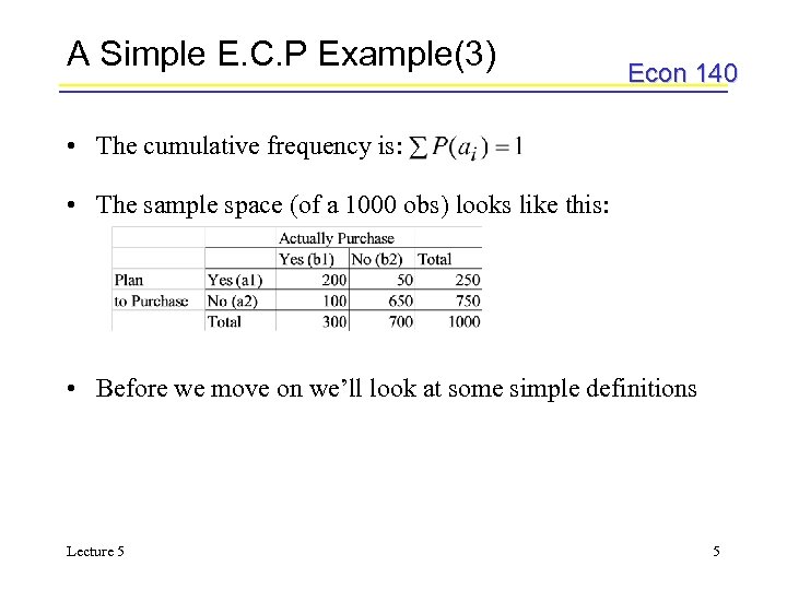
A Simple E. C. P Example(3) Econ 140 • The cumulative frequency is: • The sample space (of a 1000 obs) looks like this: • Before we move on we’ll look at some simple definitions Lecture 5 5
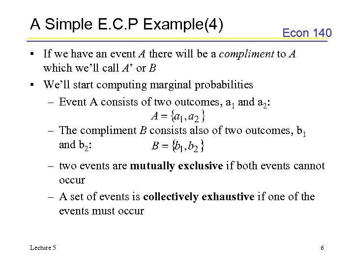
A Simple E. C. P Example(4) Econ 140 • If we have an event A there will be a compliment to A which we’ll call A’ or B • We’ll start computing marginal probabilities – Event A consists of two outcomes, a 1 and a 2: – The compliment B consists also of two outcomes, b 1 and b 2: – two events are mutually exclusive if both events cannot occur – A set of events is collectively exhaustive if one of the events must occur Lecture 5 6
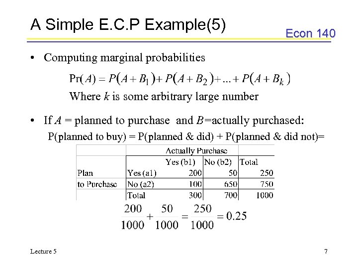
A Simple E. C. P Example(5) Econ 140 • Computing marginal probabilities Where k is some arbitrary large number • If A = planned to purchase and B=actually purchased: P(planned to buy) = P(planned & did) + P(planned & did not)= Lecture 5 7
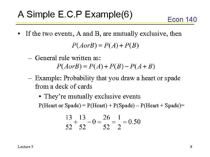
A Simple E. C. P Example(6) Econ 140 • If the two events, A and B, are mutually exclusive, then – General rule written as: – Example: Probability that you draw a heart or spade from a deck of cards • They’re mutually exclusive events P(Heart or Spade) = P(Heart) + P(Spade) – P(Heart + Spade)= Lecture 5 8
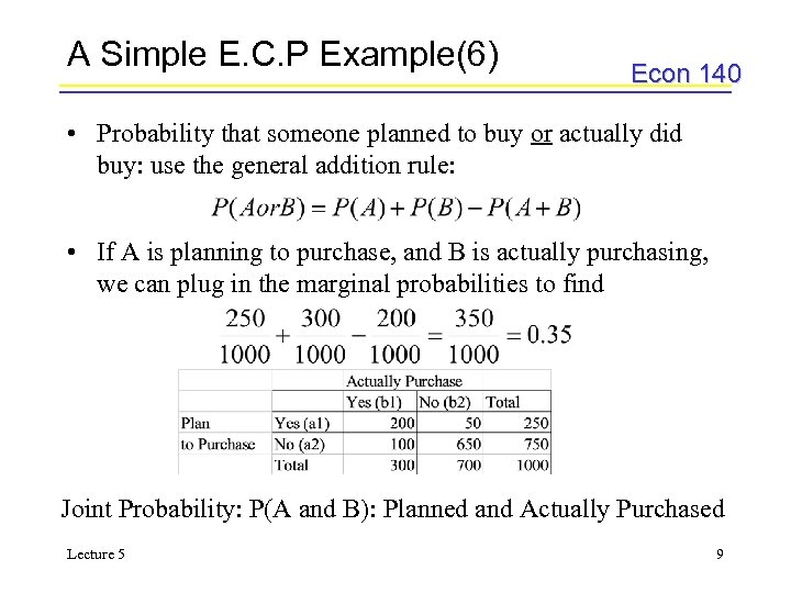
A Simple E. C. P Example(6) Econ 140 • Probability that someone planned to buy or actually did buy: use the general addition rule: • If A is planning to purchase, and B is actually purchasing, we can plug in the marginal probabilities to find Joint Probability: P(A and B): Planned and Actually Purchased Lecture 5 9
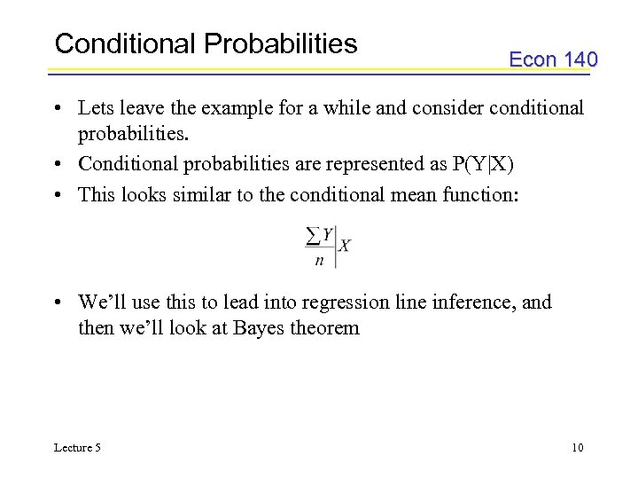
Conditional Probabilities Econ 140 • Lets leave the example for a while and consider conditional probabilities. • Conditional probabilities are represented as P(Y|X) • This looks similar to the conditional mean function: • We’ll use this to lead into regression line inference, and then we’ll look at Bayes theorem Lecture 5 10
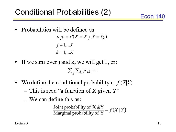
Conditional Probabilities (2) Econ 140 • Probabilities will be defined as • If we sum over j and k, we will get 1, or: • We define the conditional probability as f (X|Y) – This is read “a function of X given Y” – We can define this as: Lecture 5 11
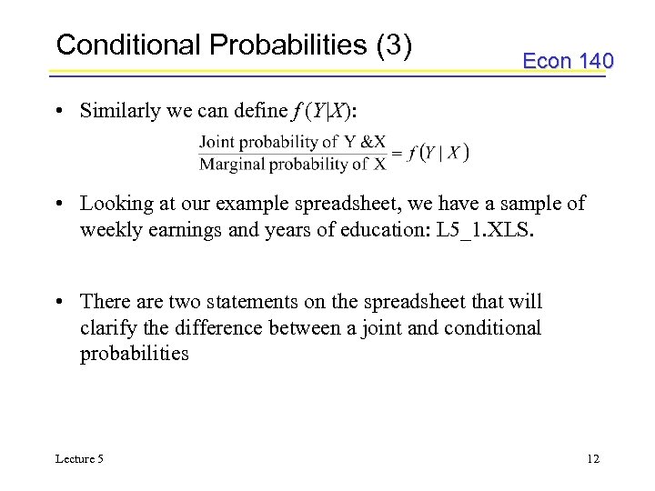
Conditional Probabilities (3) Econ 140 • Similarly we can define f (Y|X): • Looking at our example spreadsheet, we have a sample of weekly earnings and years of education: L 5_1. XLS. • There are two statements on the spreadsheet that will clarify the difference between a joint and conditional probabilities Lecture 5 12
Conditional Probabilities (4) Econ 140 • The joint probability is a relative frequency and it asks: – How many people earn between $600 and $799 and have 10 years of education? • The conditional probability asks: – How many people earn between $600 and $799 given they have 10 years of education? • On the spreadsheet I’ve outlined the cells that contain the highest probability in each completed years of education – There’s a pattern you should notice Lecture 5 13
Conditional Probabilities (5) Econ 140 • We can use the same data to graph the conditional mean function – the graph shows the same pattern we saw in the outlined cells – The conditional probability table gives us a small distribution around each year of education Lecture 5 14
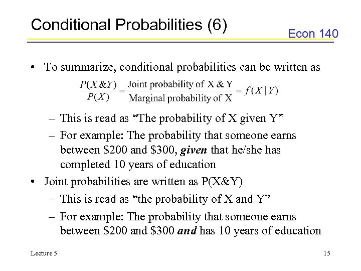
Conditional Probabilities (6) Econ 140 • To summarize, conditional probabilities can be written as – This is read as “The probability of X given Y” – For example: The probability that someone earns between $200 and $300, given that he/she has completed 10 years of education • Joint probabilities are written as P(X&Y) – This is read as “the probability of X and Y” – For example: The probability that someone earns between $200 and $300 and has 10 years of education Lecture 5 15
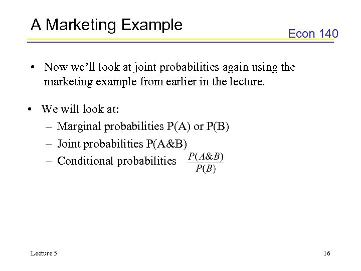
A Marketing Example Econ 140 • Now we’ll look at joint probabilities again using the marketing example from earlier in the lecture. • We will look at: – Marginal probabilities P(A) or P(B) – Joint probabilities P(A&B) – Conditional probabilities Lecture 5 16
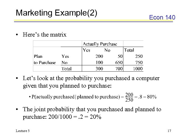
Marketing Example(2) Econ 140 • Here’s the matrix • Let’s look at the probability you purchased a computer given that you planned to purchase: • The joint probability that you purchased and planned to purchase: 200/1000 =. 2 = 20% Lecture 5 17
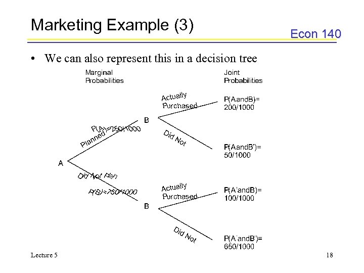
Marketing Example (3) Econ 140 • We can also represent this in a decision tree Lecture 5 18
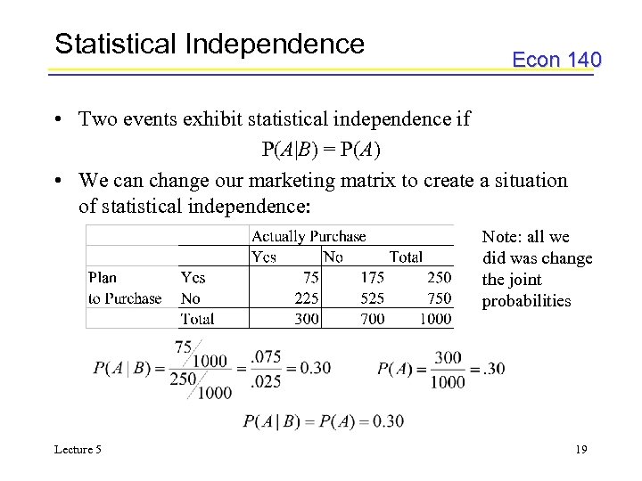
Statistical Independence Econ 140 • Two events exhibit statistical independence if P(A|B) = P(A) • We can change our marketing matrix to create a situation of statistical independence: Note: all we did was change the joint probabilities Lecture 5 19
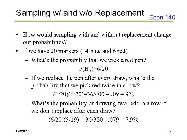
Sampling w/ and w/o Replacement Econ 140 • How would sampling with and without replacement change our probabilities? • If we have 20 markers (14 blue and 6 red) – What’s the probability that we pick a red pen? P(BR)=6/20 – If we replace the pen after every draw, what’s the probability that we pick red twice in a row? (6/20)=36/400 =. 09 = 9% – What’s the probability of drawing two reds in a row if we don’t replace after each draw? (6/20)(5/19) = 30/380 =. 079 = 7. 9% Lecture 5 20
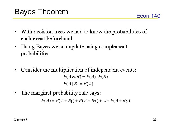
Bayes Theorem Econ 140 • With decision trees we had to know the probabilities of each event beforehand • Using Bayes we can update using complement probabilities • Consider the multiplication of independent events: • The marginal probability rule says: Lecture 5 21
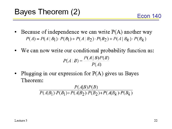
Bayes Theorem (2) Econ 140 • Because of independence we can write P(A) another way • We can now write our conditional probability function as: • Plugging in our expression for P(A) gives us Bayes Theorem: Lecture 5 22
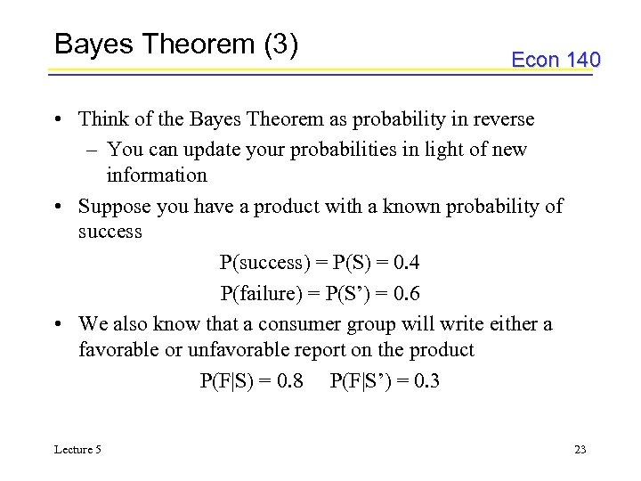
Bayes Theorem (3) Econ 140 • Think of the Bayes Theorem as probability in reverse – You can update your probabilities in light of new information • Suppose you have a product with a known probability of success P(success) = P(S) = 0. 4 P(failure) = P(S’) = 0. 6 • We also know that a consumer group will write either a favorable or unfavorable report on the product P(F|S) = 0. 8 P(F|S’) = 0. 3 Lecture 5 23
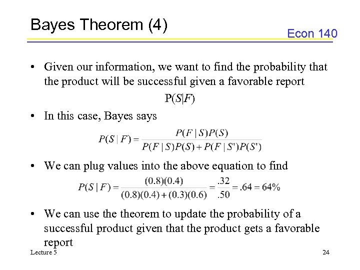
Bayes Theorem (4) Econ 140 • Given our information, we want to find the probability that the product will be successful given a favorable report P(S|F) • In this case, Bayes says • We can plug values into the above equation to find • We can use theorem to update the probability of a successful product given that the product gets a favorable report Lecture 5 24
Recap Econ 140 • We’ve seen how we can calculate marginal, joint, and conditional probabilities – Computer company example – Spreadsheet: L 5_1. XLS • We talked about statistical independence • We’ve seen how Bayes Theorem allows us to update our priors Lecture 5 25
b60b4209313f42572da6268bad3da236.ppt