Econ 100 Lecture 10 How a tax imposed

Econ 100 Lecture 10 How a tax imposed on the sales of a specific good affects the total surplus generated in the market for that good: Taxation and Market Efficiency

In the last lecture, we have seen that the price and the quantity in the equilibrium of a perfectly competitive market maximize the total surplus derived by buyers and sellers. We have also seen that, if there are no externalities associated with the production and consumption of the good bought and sold in that market, the price and the quantity in the equilibrium of a perfectly competitive market maximize also the total surplus for the society. This implies that, if any factor causes the market outcome to deviate from the equilibrium, some of the total surplus will be lost (efficiency loss or welfare loss).

An example would be a tax imposed on the sales of the good. A tax will cause the price and the quantity in a market deviate from the price and quantity in the equilibrium of the market that would arise in the absence of the tax, and therefore it will cause some welfare loss. Taxes are imposed for several reasons. One of them is that the government needs to raise some revenue to cover its expenditures that it will make when providing, for example, public services which have their benefits or the people.

The welfare loss due to a taxes imposed in the markets for specific goods can be seen as the cost of, for example, providing those public services by making the necessary expenditures using the revenue raised by imposing taxes.

Review: Effect of the tax on the market outcome In one of the previous lectures, we have seen that the imposition of a tax of the amount T per unit of a specific good causes the price paid by the buyers to increase (from Pe to Pb) the price received by the sellers to decrease (from Pe to Ps) the quantity produced and sold to decrease (from Qe to Q*) such that Ps < Pe < Pb and Pb – Ps = T, regardless of whether T is imposed on buyers and sellers.

Effect of the tax on the market efficiency (welfare effect) Once we make the observation that the tax causes Q to decrease from Qe to Q*, we can immediately tell that some of the total surplus will be lost (or not realized), and the amount of the total surplus lost will be given by the area that lies under the D curve, above the S curve, and between Q* and Qe. The amount of the total surplus lost measured by this roughly triangular area is called the “deadweight loss” (DWL).

It is called the deadweight loss because it is lost as a result of the act of transferring the tax revenue from buyers and sellers to the government, just like, during the transportation of any load, the weight of the vehicle (ship, truck etc) used to carry the load has to be carried together with the load which costs extra fuel and energy and that's a loss. Now, even though it is already clear that there will be some net loss of total surplus, we should look at the details to see how this loss is shared between the buyers, the sellers, and the government.

This requires us to examine the effect of the tax on the consumer surplus as well as on the producer surplus. Let us first draw the D and S curves for a specific good and define the following areas: Area A (triangular) = area under the D curve, above Pb, and between 0 and Q* units Area B (rectangular) = area under Pb, above Pe, and between 0 and Q* units Area C (triangular) = area under the D curve, above Pe, and between Q* and Qe units

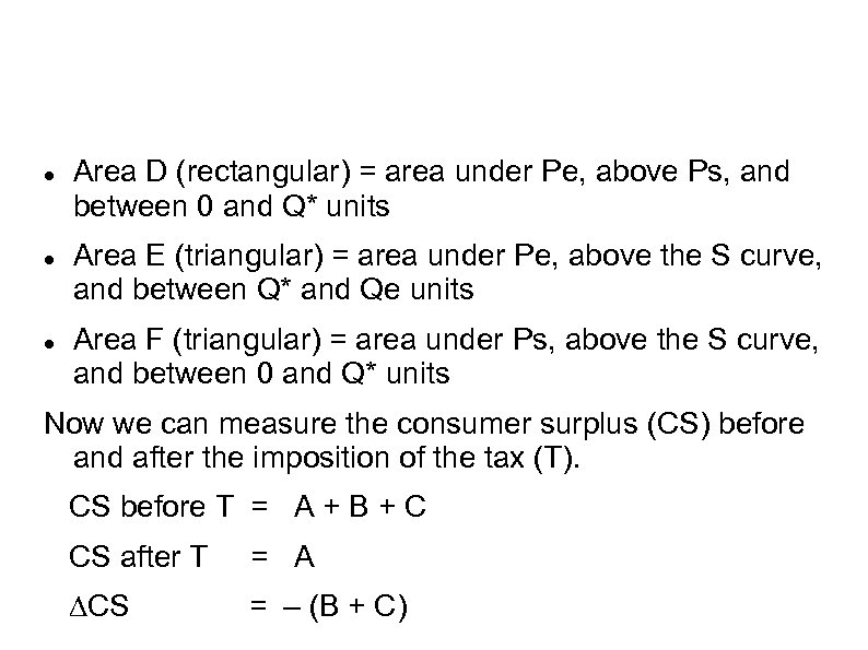Area D (rectangular) = area under Pe, above Ps, and between 0 and Q* units Area E (triangular) = area under Pe, above the S curve, and between Q* and Qe units Area F (triangular) = area under Ps, above the S curve, and between 0 and Q* units Now we can measure the consumer surplus (CS) before and after the imposition of the tax (T). CS before T = A + B + C CS after T = A ∆CS = – (B + C)

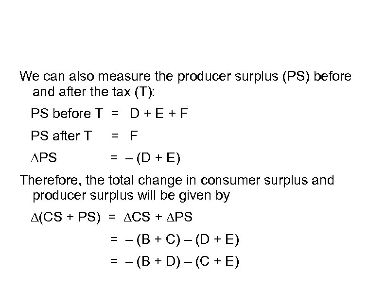We can also measure the producer surplus (PS) before and after the tax (T): PS before T = D + E + F PS after T = F ∆PS = – (D + E) Therefore, the total change in consumer surplus and producer surplus will be given by ∆(CS + PS) = ∆CS + ∆PS = – (B + C) – (D + E) = – (B + D) – (C + E)

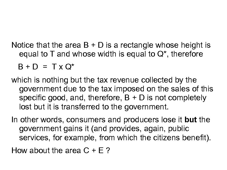Notice that the area B + D is a rectangle whose height is equal to T and whose width is equal to Q*, therefore B + D = T x Q* which is nothing but the tax revenue collected by the government due to the tax imposed on the sales of this specific good, and, therefore, B + D is not completely lost but it is transferred to the government. In other words, consumers and producers lose it but the government gains it (and provides, again, public services, for example, from which the citizens benefit). How about the area C + E ?

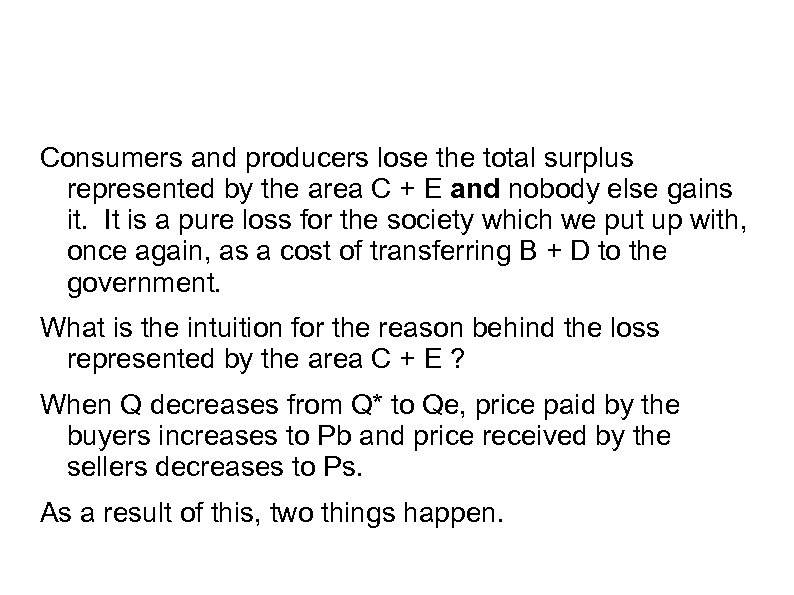Consumers and producers lose the total surplus represented by the area C + E and nobody else gains it. It is a pure loss for the society which we put up with, once again, as a cost of transferring B + D to the government. What is the intuition for the reason behind the loss represented by the area C + E ? When Q decreases from Q* to Qe, price paid by the buyers increases to Pb and price received by the sellers decreases to Ps. As a result of this, two things happen.

First, for all the buyers who would buy the units between Q* to Qe, the maximum willingness to pay for (the value the buyers subjectively place on) such units of the good is less than Pb so they don't buy any units. Second, for all the sellers who would produce and sell the units between Q* and Qe, the cost is more than Ps so they don't produce and sell any units. As a result of these, the total surrplus that would be realized from the production and sale of any unit between Q* and Qe is not realized, and it is forgone or lost.

What the size of the deadweight loss depends on Consider the D and S curves for a good on whose sales a tax T is imposed and the area representing the DWL. The size of the DWL will depend on the price elasticities of D and S curves. Notice that, as D and T remain the same but S becomes more elastic, DWL increases. Notice also that, as S and T remain the same but D becomes more elastic, DWL increases.

How the size of the deadweight loss changes as the tax per unit changes Consider again the D and S curves for a good on whose sales a tax T is imposed and the area representing the DWL. The size of the DWL also depends on T. Notice that as the D and S curves remain the same but T increases, Qe – Q* increases and DWL increases. Notice also that, as T increases, DWL increases at an increasing rate so that the slope of the curve which is the graph of the relationship between DWL and T is increasing (the curve becoming steeper), and the relationship between DWL and T is not linear but roughly quadratic. Why?

How the tax revenue changes as the tax per unit changes (the so-called “Laffer curve”) As T increases, there will be a positive effect on the tax revenue because T is a factor in the multiplication T x Q*. At the same time, Q* will decrease as T increases, and there will be a negative effect on the tax revenue because Q* is also a factor in the multiplication T x Q*. Then, what will be the net effect on the tax revenue? Will it increase or decrease as T increases? To find the answer to this question, consider alternative values for T starting from 0.

When T = 0, there is no effect on Q but the tax revenue T x Q is zero because T = 0. Now consider the maximum possible value of T. T can be so large that Q is reduced to 0. Then, T x Q is zero again, this time because Q = 0. In between, there are some values of T such that 0 < Qe so that T x Q is positive. These observations suggest that, as T increases starting from 0, T x Q starts from 0, increases to some positive value, and then it begins to decrease sooner or later, because it will finally drop to 0 when T reaches its maximum value.

This implies that the graph of the relationship between the tax revenue and the tax per unit would be a curve which is first increasing and then decreasing, reaching a maximum (at least one) in between. This, in turn, implies that the same tax revenue can be collected by imposing at least two different T values (one relatively low, the other high), and raising T beyond a certain value will reduce T x Q, or lowering T from some value which is close enough to the highest value of T will first make T x Q increase instead of decrease.