ECODE FP 7 Project Training Seminar Session 2

ECODE FP 7 Project Training Seminar: Session 2 a Internet architecture (incl. Topology structure, and models) Dimitri Papadimitriou and Olivier Bonaventure Alcatel-Lucent BELL - Universite catholique de Louvain (UCL) September 1, 2008 Alcatel-Lucent BELL Antwerpen, Belgium

Outline 1. Organization of the Internet Topology Types of domains – – – Transit domain Stub domain Example of domains Internet Routing 2. Evolution of the Internet Number of Hosts IP address allocation – – IPv 4 address allocation IPv 6 address allocation Size of the IPv 4 BGP routing tables Size of the IPv 6 BGP routing tables Number of AS Routing tables IP traffic flows Bandwidth

Outline 3. Internet Topology modelling Network properties Random Graphs models and generators Structural models and generators Topology measurements Power Law relationships Degree-based models and generators Internet topology metrics

Outline 1. Organization of the Internet Topology Types of domains – – – Transit domain Stub domain Example of domains Internet Routing 2. Evolution of the Internet 3. Internet Topology modeling

Organization of the Internet § Internet: infrastructure composed by an interconnected set of (heterogeneous) networks architected around a distributed routing system that is partitioned into independently administrated domains (autonomous systems) § A domain is a set of routers, links, hosts and local area networks under the same administrative control A domain can be very large. . . – A domain can be very small. . . – § AS 568: SUMNET-AS DISO-UNRRA contains 73154560 IP addresses AS 2111: IST-ATRIUM TE Experiment a single PC running Linux. . . Internet is composed of ~ 30. 000 autonomous systems (AS)

Organization of the Internet § Domains are interconnected in various ways The interconnection of all domains should in theory allow packets to be sent anywhere Usually IP datagram will need to cross a few ASes (3 to 4, average 3. 4) to reach its destination

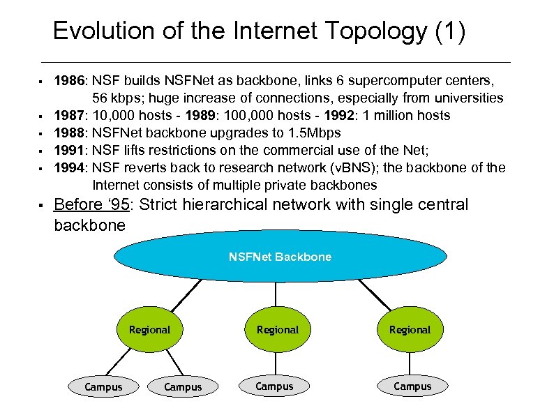Evolution of the Internet Topology (1) § § § 1986: NSF builds NSFNet as backbone, links 6 supercomputer centers, 56 kbps; huge increase of connections, especially from universities 1987: 10, 000 hosts - 1989: 100, 000 hosts - 1992: 1 million hosts 1988: NSFNet backbone upgrades to 1. 5 Mbps 1991: NSF lifts restrictions on the commercial use of the Net; 1994: NSF reverts back to research network (v. BNS); the backbone of the Internet consists of multiple private backbones Before ‘ 95: Strict hierarchical network with single central backbone NSFNet Backbone Regional Campus

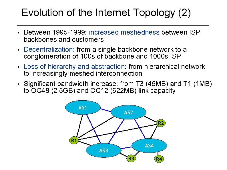Evolution of the Internet Topology (2) § § Between 1995 -1999: increased meshedness between ISP backbones and customers Decentralization: from a single backbone network to a conglomeration of 100 s of backbone and 1000 s ISP Loss of hierarchy and abstraction: from hierarchical network to increasingly meshed interconnection Significant bandwidth increase: from T 3 (45 MB) and T 1 (1 MB) to OC 48 (2. 5 GB) and OC 12 (622 MB) link capacity AS 1 AS 2 R 1 AS 4 AS 3 R 4

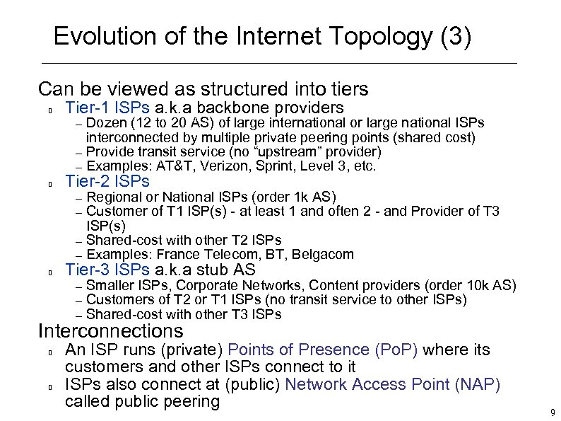Evolution of the Internet Topology (3) Can be viewed as structured into tiers Tier-1 ISPs a. k. a backbone providers – – – Dozen (12 to 20 AS) of large international or large national ISPs interconnected by multiple private peering points (shared cost) Provide transit service (no “upstream” provider) Examples: AT&T, Verizon, Sprint, Level 3, etc. Tier-2 ISPs – – Regional or National ISPs (order 1 k AS) Customer of T 1 ISP(s) - at least 1 and often 2 - and Provider of T 3 ISP(s) Shared-cost with other T 2 ISPs Examples: France Telecom, BT, Belgacom – – – Smaller ISPs, Corporate Networks, Content providers (order 10 k AS) Customers of T 2 or T 1 ISPs (no transit service to other ISPs) Shared-cost with other T 3 ISPs – – Tier-3 ISPs a. k. a stub AS Interconnections An ISP runs (private) Points of Presence (Po. P) where its customers and other ISPs connect to it ISPs also connect at (public) Network Access Point (NAP) called public peering 9

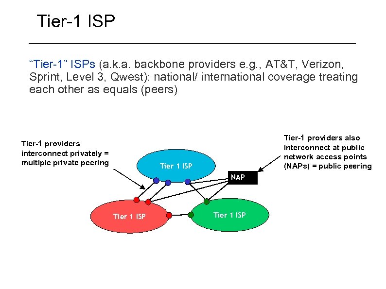Tier-1 ISP “Tier-1” ISPs (a. k. a. backbone providers e. g. , AT&T, Verizon, Sprint, Level 3, Qwest): national/ international coverage treating each other as equals (peers) Tier-1 providers interconnect privately = multiple private peering Tier-1 providers also interconnect at public network access points (NAPs) = public peering Tier 1 ISP NAP Tier 1 ISP

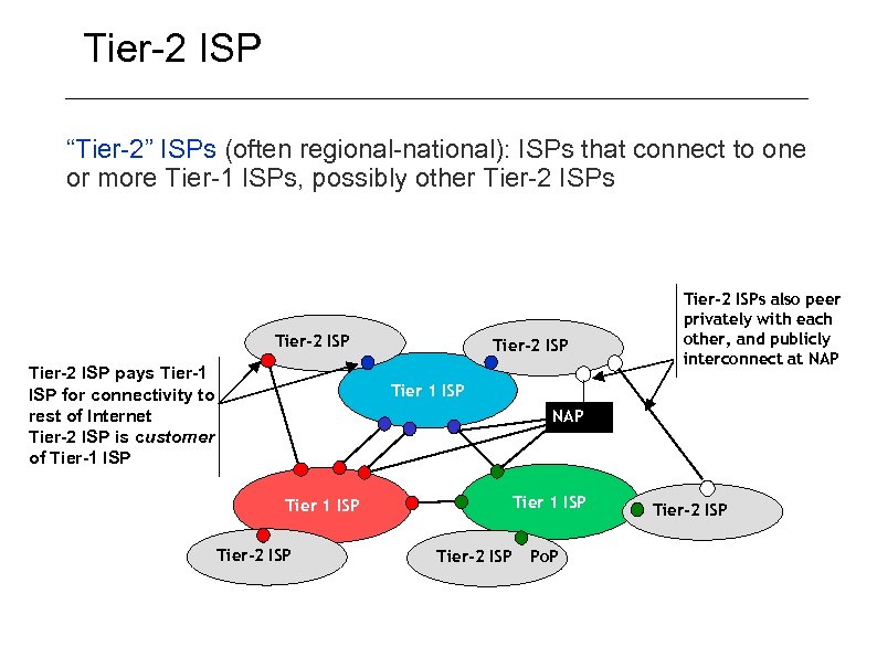Tier-2 ISP “Tier-2” ISPs (often regional-national): ISPs that connect to one or more Tier-1 ISPs, possibly other Tier-2 ISPs Tier-2 ISP pays Tier-1 ISP for connectivity to rest of Internet Tier-2 ISP is customer of Tier-1 ISP Tier-2 ISPs also peer privately with each other, and publicly interconnect at NAP Tier 1 ISP Tier-2 ISP Po. P Tier-2 ISP

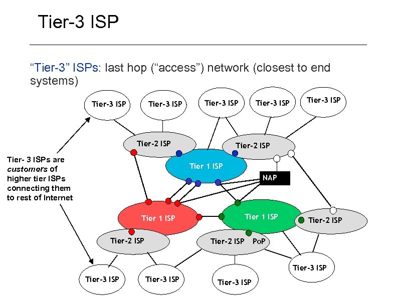Tier-3 ISP “Tier-3” ISPs: last hop (“access”) network (closest to end systems) Tier-3 ISP Tier-2 ISP Tier- 3 ISPs are customers of higher tier ISPs connecting them to rest of Internet Tier-3 ISP Tier-2 ISP Tier 1 ISP NAP Tier 1 ISP Tier-2 ISP Po. P Tier-3 ISP

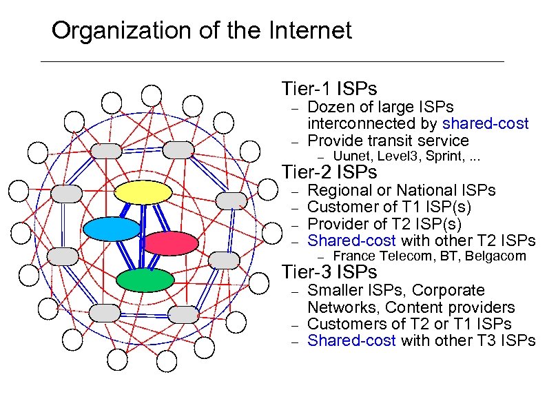Organization of the Internet Tier-1 ISPs – – Dozen of large ISPs interconnected by shared-cost Provide transit service – Uunet, Level 3, Sprint, . . . Tier-2 ISPs – – Regional or National ISPs Customer of T 1 ISP(s) Provider of T 2 ISP(s) Shared-cost with other T 2 ISPs – France Telecom, BT, Belgacom Tier-3 ISPs – – – Smaller ISPs, Corporate Networks, Content providers Customers of T 2 or T 1 ISPs Shared-cost with other T 3 ISPs

AS Ranking § Proposing two ranking methods: Degree-based: ASes are ranked by their degrees in the AS topology graph: http: //as-rank. caida. org/ AS-relationship-based: ASes are ranked by their customer cone sizes See http: //as-rank. caida. org/data Route. Views BGP AS links annotated with inferred relationships Dataset date: 20080818 Alpha parameter of inference algorithm: 0. 01000 Format: where and are AS numbers, and is -1 if AS 1 is a customer of AS 2, 0 if AS 1 and AS 2 are peers, 1 if AS 1 is a provider of AS 2, and 2 if AS 1 and AS 2 are siblings (the same organization)

Summary § Based on AS connectivity and relationships, the Internet routing infrastructure can be viewed as a three tier hierarchy Core: consisting of a dozen or so Tier-1 providers forming the top level of the hierarchy Middle: consisting of few thousands of ASes (Tier-2 providers) that provide transit service but are not part of the core Edge: 10 thousands of stub ASes that do not provide transit service. Usually, local ISP, ASP and CSP

Outline 1. Organization of the Internet Topology Types of domains – – – Transit domain Stub domain Example of domains Internet Routing 2. Evolution of the Internet 3. Internet Topology modeling

Types of domains § The Internet consists of routing domains: Autonomous Systems (AS) interconnected with each other: Transit domain: provider, hooking many AS together Stub domain: smaller corporation/domain: – – § At least one and usually two connections to other domain No transit service to other domains Two-level routing: Intra-domain: administrator responsible for choice of routing protocol within network (usually link-state routing protocol) Inter-domain: standard for interdomain routing: BGP

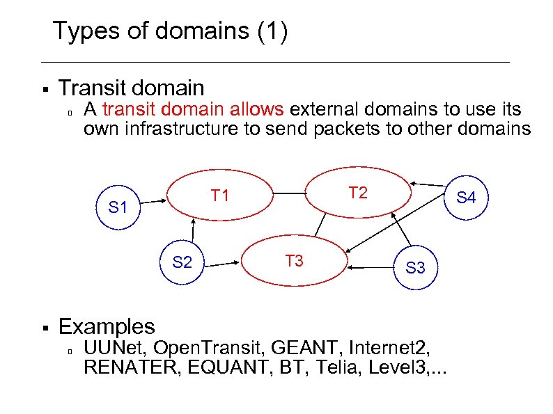Types of domains (1) § Transit domain A transit domain allows external domains to use its own infrastructure to send packets to other domains S 1 S 2 § Examples T 2 T 1 T 3 S 4 S 3 UUNet, Open. Transit, GEANT, Internet 2, RENATER, EQUANT, BT, Telia, Level 3, . . .

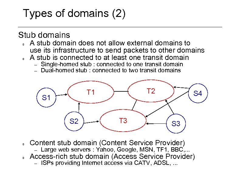Types of domains (2) Stub domains A stub domain does not allow external domains to use its infrastructure to send packets to other domains A stub is connected to at least one transit domain – – Single-homed stub : connected to one transit domain Dual-homed stub : connected to two transit domains S 1 S 2 T 2 T 1 T 3 S 4 S 3 Content stub domain (Content Service Provider) – Large web servers : Yahoo, Google, MSN, TF 1, BBC, . . . – ISPs providing Internet access via CATV, ADSL, . . . Access-rich stub domain (Access Service Provider)

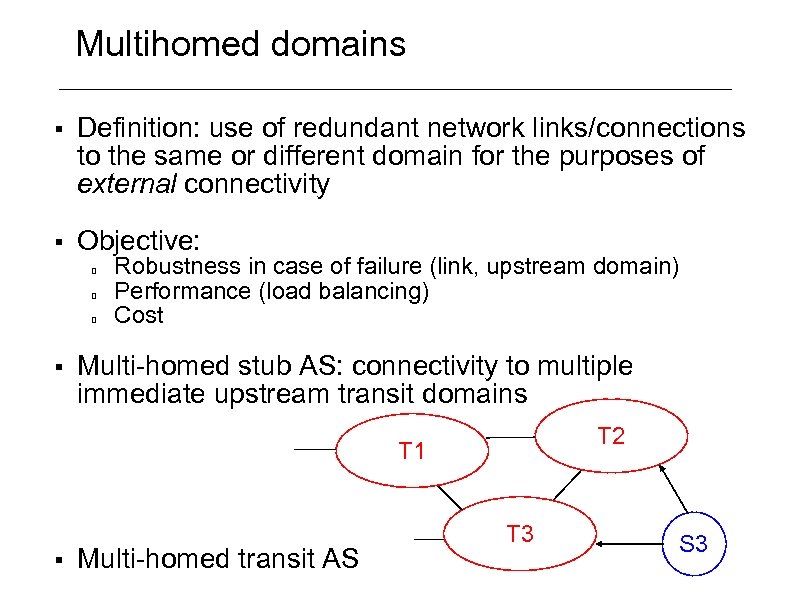Multihomed domains § Definition: use of redundant network links/connections to the same or different domain for the purposes of external connectivity § Objective: § Robustness in case of failure (link, upstream domain) Performance (load balancing) Cost Multi-homed stub AS: connectivity to multiple immediate upstream transit domains T 2 T 1 § Multi-homed transit AS T 3 S 3

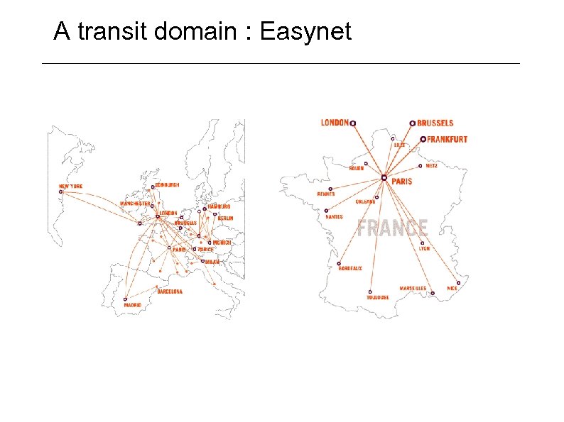A transit domain : Easynet

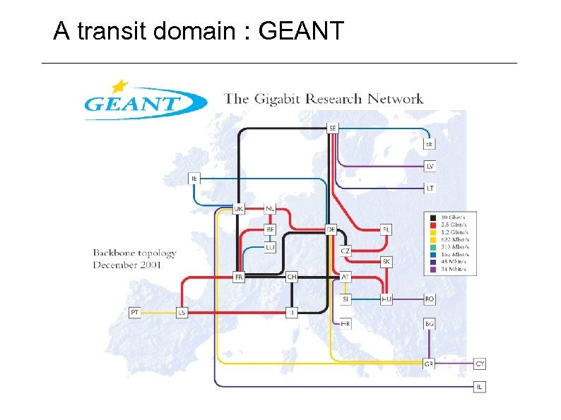A transit domain : GEANT

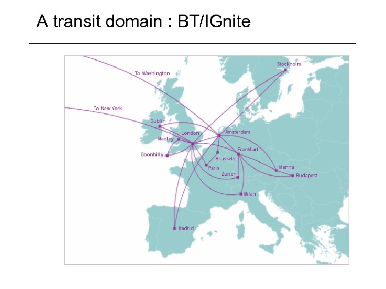A transit domain : BT/IGnite

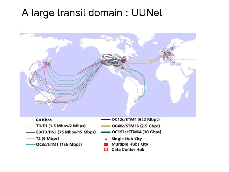A large transit domain : UUNet

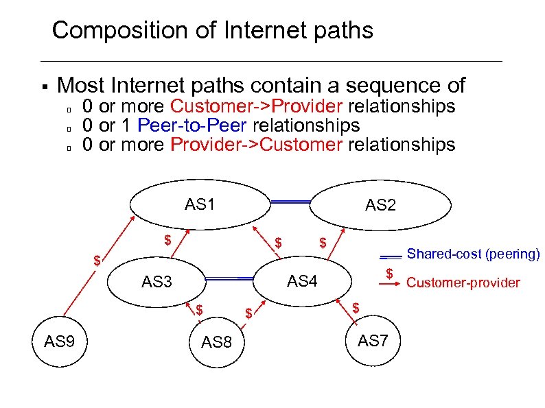Composition of Internet paths § Most Internet paths contain a sequence of 0 or more Customer->Provider relationships 0 or 1 Peer-to-Peer relationships 0 or more Provider->Customer relationships AS 1 AS 2 $ $ $ Shared-cost (peering) $ $ AS 9 $ AS 4 AS 3 AS 8 $ $ AS 7 Customer-provider

Outline 1. Organization of the Internet Topology Types of domains – – – Transit domain Stub domain Example of domains Internet Routing 2. Evolution of the Internet 3. Internet Topology modeling

Internet Routing Internet domains comprises devices called routers comprising a routing and a forwarding engine (and a management agent) Routing engine: Process routing information (exchanged between routers using a routing protocols such as BGP) so as to compute routes (using a shortest path algorithms) Routes entries (composed by a destination, a next-hop interface, and a metric) are stored in routing information bases (RIB) Routing entries are subsequently used by the forwarding engine Forwarding engine: Transfer incoming IP datagram to an outgoing interface directed towards a router closer (next-hop) to the traffic destination by performing a longest match prefix lookup on forwarding entries stored in forwarding information base (FIB) using the incoming IP datagram destination address

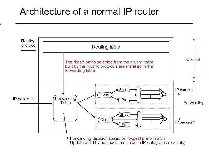Architecture of a normal IP router Routing protocol Routing table Control The "best" paths selected from the routing table built by the routing protocols are installed in the forwarding table Shap. IP packets Forwarding Table IP packets Class. Pol Forwarding Shap. Class. Pol IP packets Forwarding decision based on longest prefix match Update of TTL and checksum fields in IP datagrams (packets)

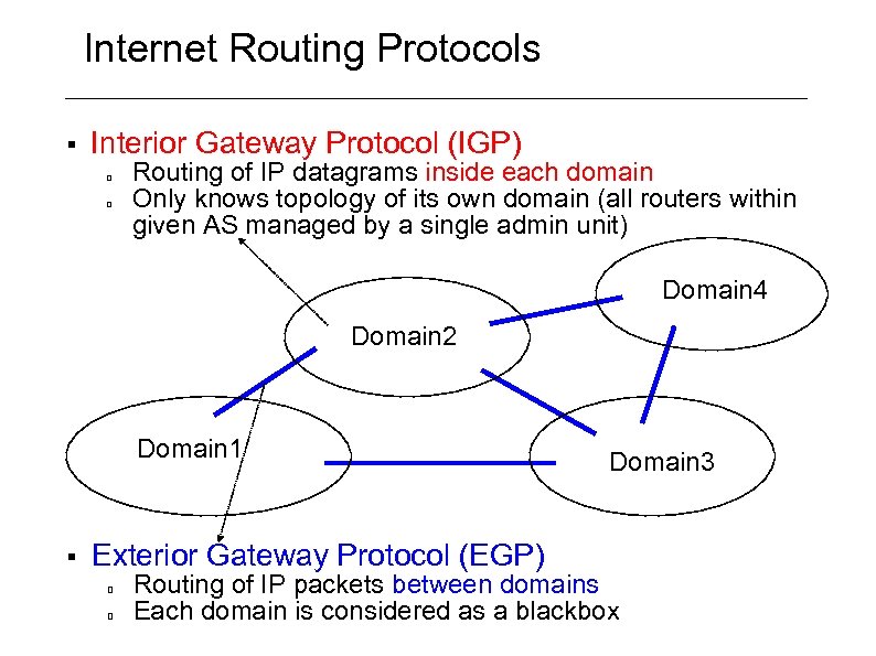Internet Routing Protocols § Interior Gateway Protocol (IGP) Routing of IP datagrams inside each domain Only knows topology of its own domain (all routers within given AS managed by a single admin unit) Domain 4 Domain 2 Domain 1 § Exterior Gateway Protocol (EGP) Domain 3 Routing of IP packets between domains Each domain is considered as a blackbox

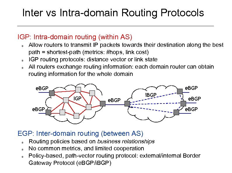Inter vs Intra-domain Routing Protocols IGP: Intra-domain routing (within AS) Allow routers to transmit IP packets towards their destination along the best path = shortest-path (metrics: #hops, link cost) IGP routing protocols: distance vector or link state All routers exchange routing information: each domain router can obtain routing information for the whole domain e. BGP IGP e. BGP i. BGP e. BGP EGP: Inter-domain routing (between AS) Routing policies based on business relationships No common metrics, and limited cooperation Policy-based, path-vector routing protocol: external/internal Border Gateway Protocol (e. BGP/i. BGP)

Session 2 a - Outline 1. Organization of the Internet 2. Evolution of the Internet Number of Hosts IP address allocation – – IPv 4 address allocation IPv 6 address allocation Size of the IPv 4 BGP routing tables Size of the IPv 6 BGP routing tables Number of AS Routing tables IP traffic flows Bandwidth 3. Internet Topology modelling

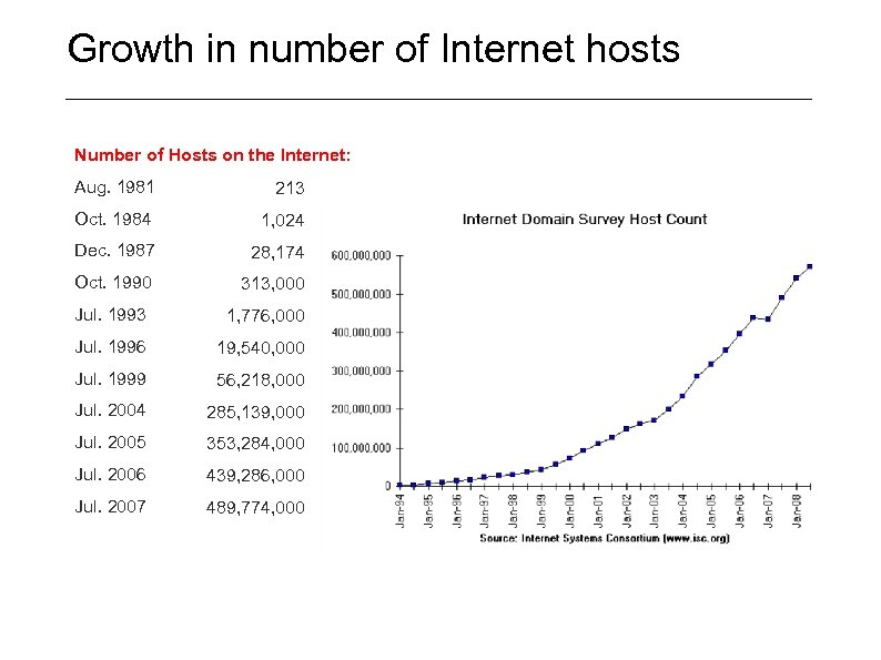Growth in number of Internet hosts Number of Hosts on the Internet: Aug. 1981 213 Oct. 1984 1, 024 Dec. 1987 28, 174 Oct. 1990 313, 000 Jul. 1993 1, 776, 000 Jul. 1996 19, 540, 000 Jul. 1999 56, 218, 000 Jul. 2004 285, 139, 000 Jul. 2005 353, 284, 000 Jul. 2006 439, 286, 000 Jul. 2007 489, 774, 000

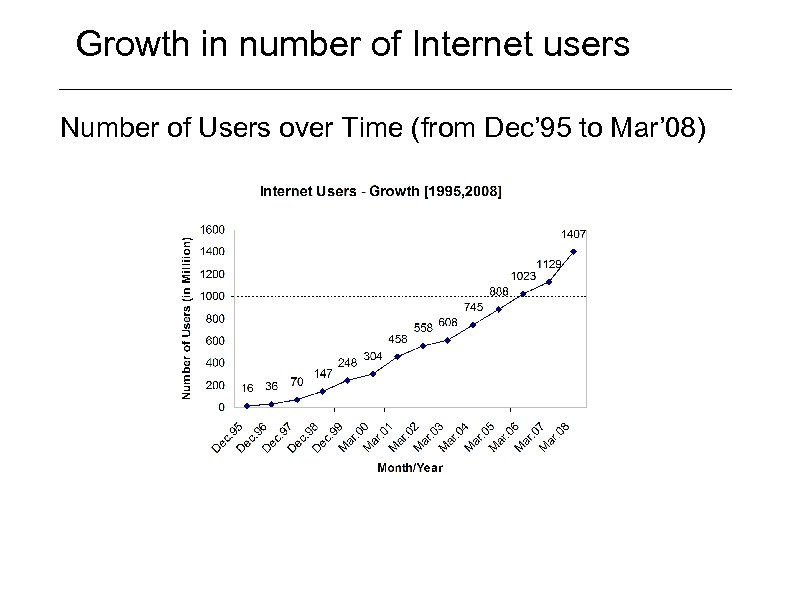Growth in number of Internet users Number of Users over Time (from Dec’ 95 to Mar’ 08)

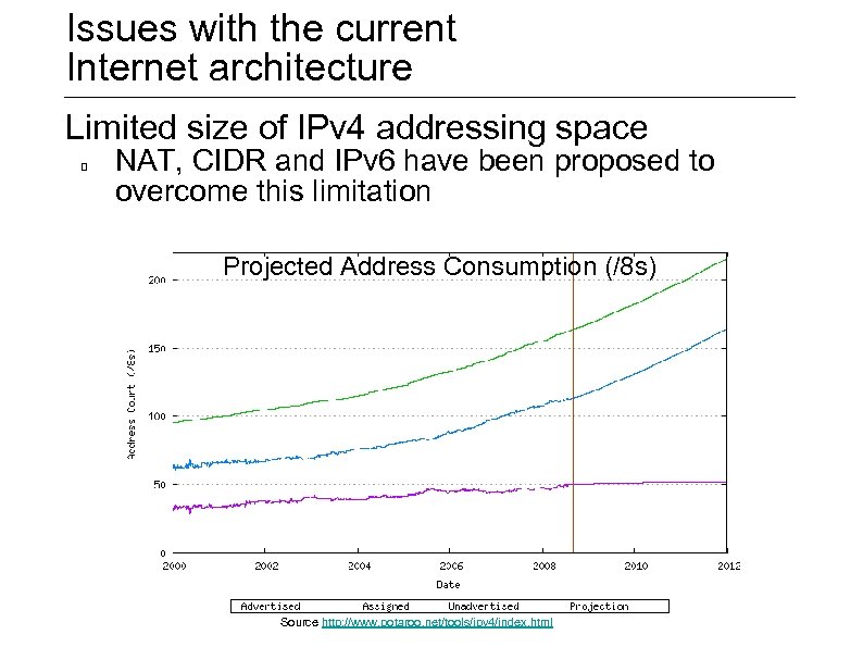Issues with the current Internet architecture Limited size of IPv 4 addressing space NAT, CIDR and IPv 6 have been proposed to overcome this limitation Projected Address Consumption (/8 s) Source http: //www. potaroo. net/tools/ipv 4/index. html

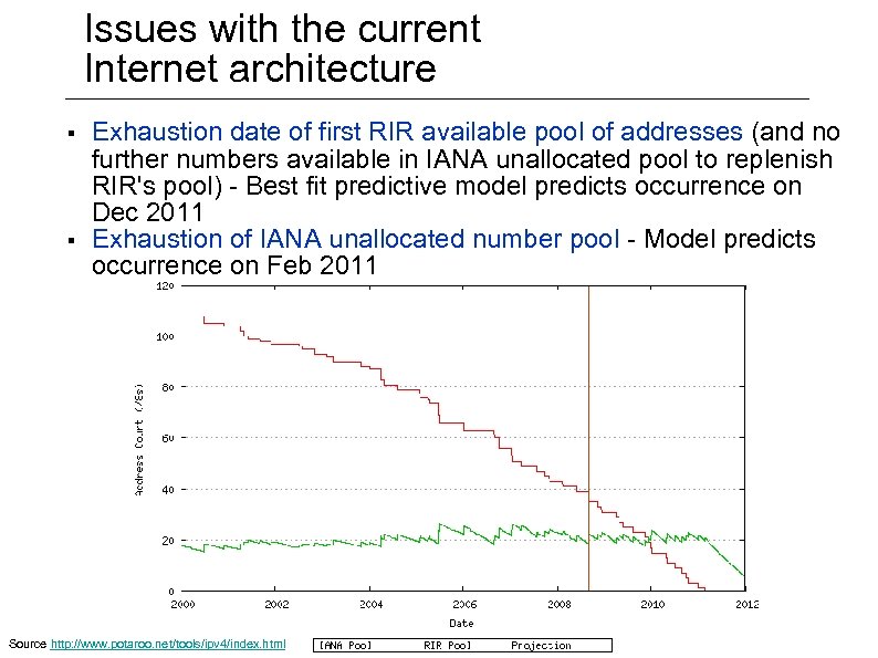Issues with the current Internet architecture § § Exhaustion date of first RIR available pool of addresses (and no further numbers available in IANA unallocated pool to replenish RIR's pool) - Best fit predictive model predicts occurrence on Dec 2011 Exhaustion of IANA unallocated number pool - Model predicts occurrence on Feb 2011 Source http: //www. potaroo. net/tools/ipv 4/index. html

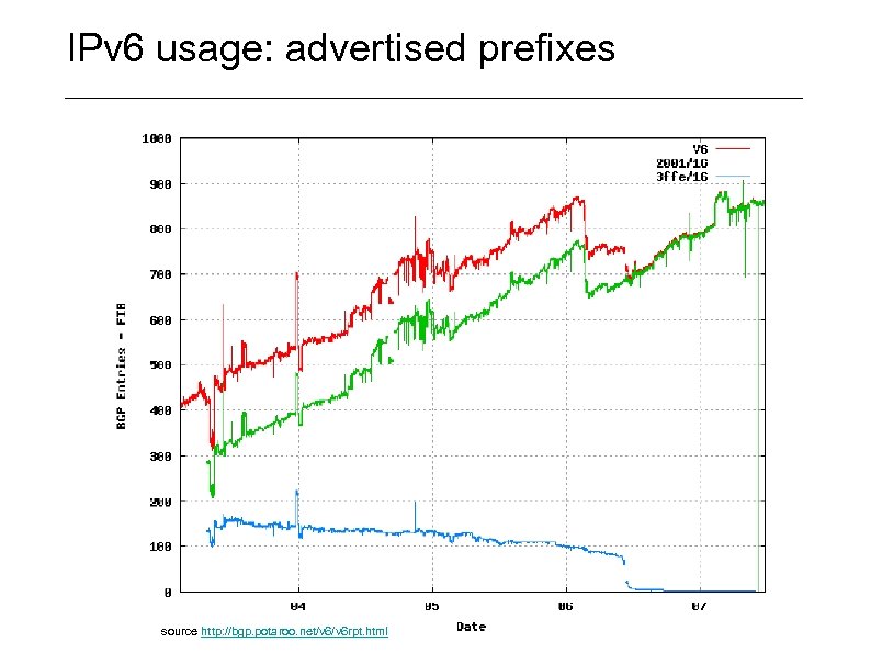IPv 6 usage: advertised prefixes source http: //bgp. potaroo. net/v 6 rpt. html

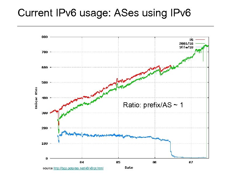Current IPv 6 usage: ASes using IPv 6 Ratio: prefix/AS ~ 1 source http: //bgp. potaroo. net/v 6 rpt. html

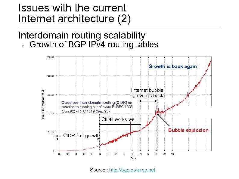Issues with the current Internet architecture (2) Interdomain routing scalability Growth of BGP IPv 4 routing tables Growth is back again ! Internet bubble: growth is back Classless Inter-domain routing (CIDR) as reaction to running out of class B: RFC 1338 (Jun. 92) - RFC 1519 (Sep. 93) CIDR works well Bubble explosion pre-CIDR fast growth Source : http: //bgp. potaroo. net

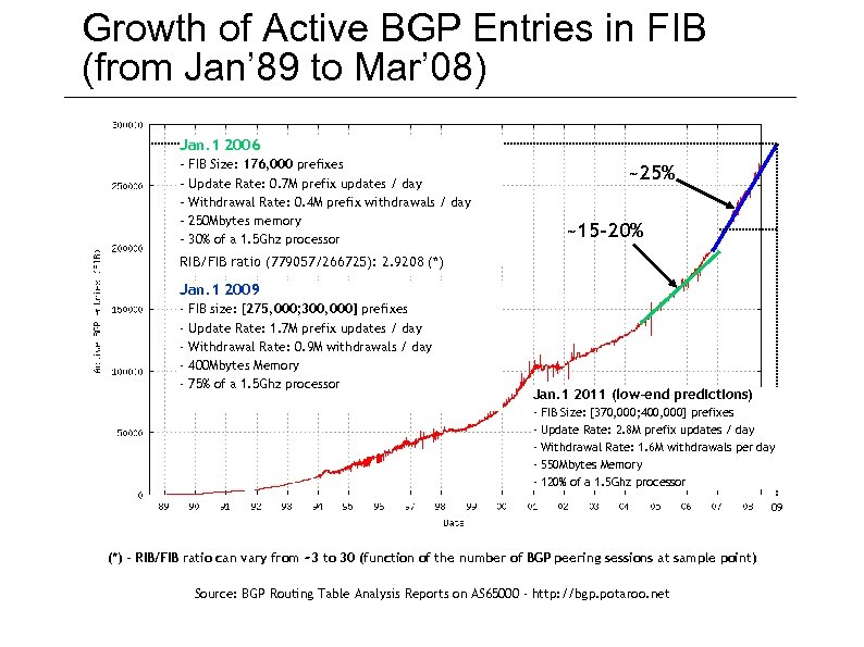Growth of Active BGP Entries in FIB (from Jan’ 89 to Mar’ 08) Jan. 1 2006 – – – FIB Size: 176, 000 prefixes Update Rate: 0. 7 M prefix updates / day Withdrawal Rate: 0. 4 M prefix withdrawals / day 250 Mbytes memory 30% of a 1. 5 Ghz processor ~25% ~15 -20% RIB/FIB ratio (779057/266725): 2. 9208 (*) Jan. 1 2009 - FIB size: [275, 000; 300, 000] prefixes Update Rate: 1. 7 M prefix updates / day Withdrawal Rate: 0. 9 M withdrawals / day 400 Mbytes Memory 75% of a 1. 5 Ghz processor Jan. 1 2011 (low-end predictions) - FIB Size: [370, 000; 400, 000] prefixes Update Rate: 2. 8 M prefix updates / day Withdrawal Rate: 1. 6 M withdrawals per day 550 Mbytes Memory 120% of a 1. 5 Ghz processor 09 (*) - RIB/FIB ratio can vary from ~3 to 30 (function of the number of BGP peering sessions at sample point) Source: BGP Routing Table Analysis Reports on AS 65000 - http: //bgp. potaroo. net

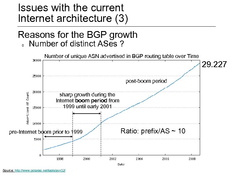Issues with the current Internet architecture (3) Reasons for the BGP growth Number of distinct ASes ? Number of unique ASN advertised in BGP routing table over Time 29. 227 post-boom period sharp growth during the Internet boom period from 1999 until early 2001 pre-Internet boom prior to 1999 Source: http: //www. potaroo. net/tools/asn 32/ Ratio: prefix/AS ~ 10

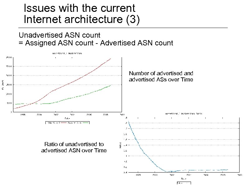Issues with the current Internet architecture (3) Unadvertised ASN count = Assigned ASN count - Advertised ASN count Number of advertised and advertised ASs over Time Ratio of unadvertised to advertised ASN over Time

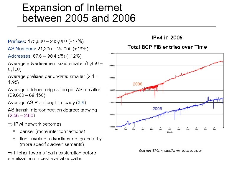Expansion of Internet between 2005 and 2006 Prefixes: 173, 800 – 203, 800 (+17%) AS Numbers: 21, 200 – 24, 000 (+13%) IPv 4 in 2006 Total BGP FIB entries over Time Addresses: 87. 6 – 98. 4 (/8) (+12%) Average advertisement size: smaller (8, 450 – 8, 100) Average prefixes per update: smaller (2. 1 1. 95) Average address origination per AS: smaller (69, 600 – 69, 150) Average AS Path length: steady (3. 4) AS transit interconnection degree: growing (2. 56 – 2. 60) IPv 4 network becomes § denser (more interconnections) § finer levels of advertisement granularity (more specific advertisements) Higher levels of path exploration before stabilization on best available paths Source: IEPG,

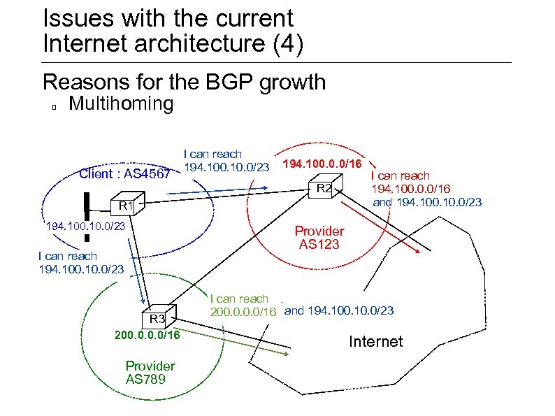Issues with the current Internet architecture (4) Reasons for the BGP growth Multihoming Client : AS 4567 I can reach 194. 100. 10. 0/23 194. 100. 0. 0/16 R 2 R 1 194. 100. 10. 0/23 I can reach 194. 100. 10. 0/23 R 3 200. 0/16 Provider AS 789 I can reach 194. 100. 0. 0/16 and 194. 100. 10. 0/23 Provider AS 123 I can reach 200. 0/16 and 194. 100. 10. 0/23 Internet

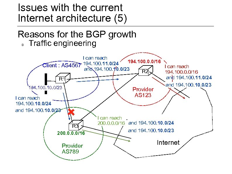Issues with the current Internet architecture (5) Reasons for the BGP growth Traffic engineering I can reach 194. 100. 0. 0/16 194. 100. 11. 0/24 Client : AS 4567 I can reach and 194. 100. 10. 0/23 R 2 194. 100. 0. 0/16 and 194. 100. 11. 0/24 R 1 and 194. 100. 10. 0/23 I can reach 194. 100. 10. 0/24 and 194. 100. 10. 0/23 R 3 200. 0/16 Provider AS 789 Provider AS 123 I can reach 200. 0/16 and 194. 100. 10. 0/24 and 194. 100. 10. 0/23 Internet

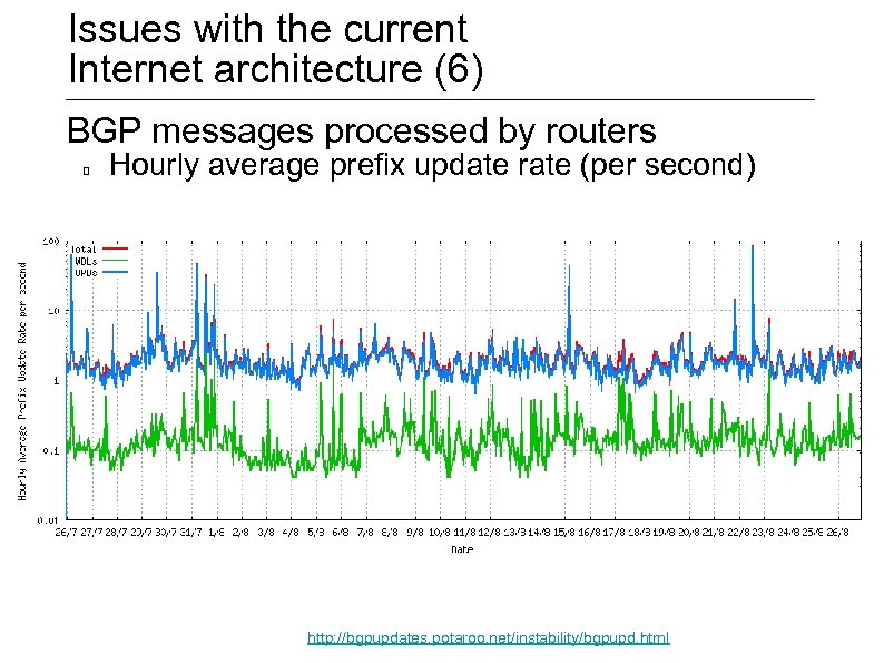Issues with the current Internet architecture (6) BGP messages processed by routers Hourly average prefix update rate (per second) http: //bgpupdates. potaroo. net/instability/bgpupd. html

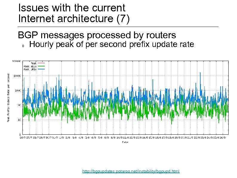Issues with the current Internet architecture (7) BGP messages processed by routers Hourly peak of per second prefix update rate http: //bgpupdates. potaroo. net/instability/bgpupd. html

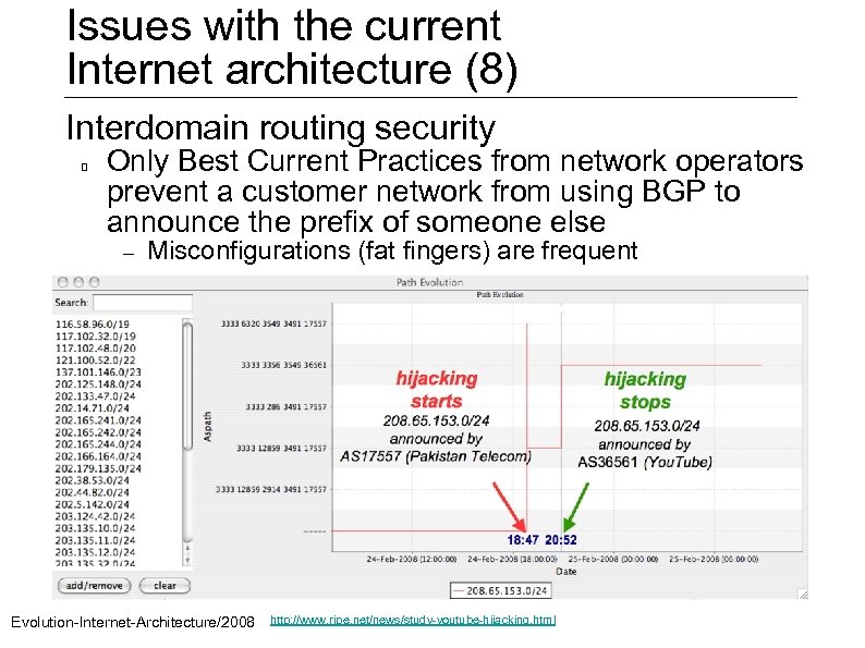Issues with the current Internet architecture (8) Interdomain routing security Only Best Current Practices from network operators prevent a customer network from using BGP to announce the prefix of someone else – Misconfigurations (fat fingers) are frequent Evolution-Internet-Architecture/2008 http: //www. ripe. net/news/study-youtube-hijacking. html

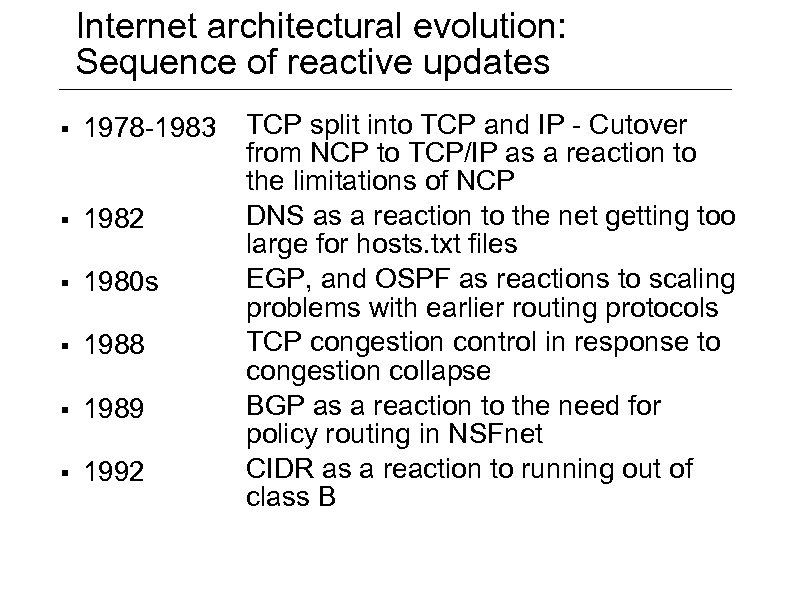Internet architectural evolution: Sequence of reactive updates § 1978 -1983 § 1982 § 1980 s § 1988 § 1989 § 1992 TCP split into TCP and IP - Cutover from NCP to TCP/IP as a reaction to the limitations of NCP DNS as a reaction to the net getting too large for hosts. txt files EGP, and OSPF as reactions to scaling problems with earlier routing protocols TCP congestion control in response to congestion collapse BGP as a reaction to the need for policy routing in NSFnet CIDR as a reaction to running out of class B

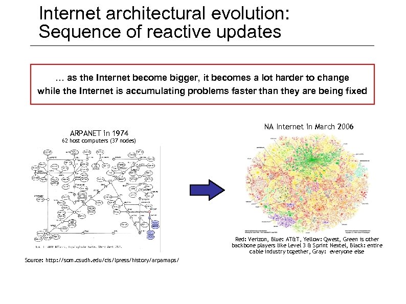Internet architectural evolution: Sequence of reactive updates … as the Internet become bigger, it becomes a lot harder to change while the Internet is accumulating problems faster than they are being fixed ARPANET in 1974 NA Internet in March 2006 62 host computers (37 nodes) Red: Verizon, Blue: AT&T, Yellow: Qwest, Green is other backbone players like Level 3 & Sprint Nextel, Black: entire cable industry together, Gray: everyone else Source: http: //som. csudh. edu/cis/lpress/history/arpamaps/

Outline 1. Organization of the Internet 2. Evolution of the Internet 3. Internet Topology modelling Network properties Random Graphs models and generators Structural models and generators Topology measurements Power Law relationships Degree-based models and generators Internet topology metrics

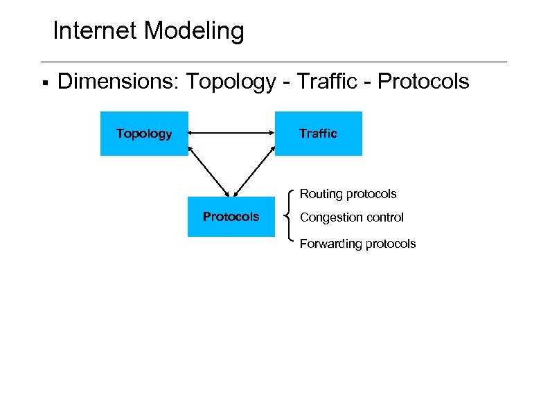Internet Modeling § Dimensions: Topology - Traffic - Protocols Topology Traffic Routing protocols Protocols Congestion control Forwarding protocols

Goals of Internet topology modeling Better understand Internet topology and its evolution Find simple fundamental properties underlying Internet “complex system” Understand why these properties appear and their effects Internet structure fundamentally affects functionality: derive Topology metrics Objectives Design more efficient routing protocols – – Because routing protocol efficiency depends on topology Simulation tools for testing old and new routing protocols – – Will the current protocols perform well in the future? How many high-class, mid-class and simple routers to produce? Create more accurate models Speculate future internet topology

Why is it important to model the network topology 1. Performance evaluation of protocols 2. Topology constrains applications and services that run on top of it Traffic engineering, capacity/resource planning, provisioning and management 3. Understanding large-scale properties Network reliability and robustness to accidents, failures and attacks on network components (security) New routing protocol design, development, and testing, e. g. of scalability, stability and convergence properties

Internet Topology modeling § Graph Representation § Most analysis considers them as un-weighted graphs Not annotated with capacity or latency Internet topology graphs: two levels of granularity Router level modeling router graphs Inter-domain level modeling AS graphs

Internet Topology modeling 1. Router-level modeling Router-level adjacencies graph – Vertices/nodes represent routers – Edges represent one-hop IP connectivity Examples – Waxman (Waxman 1988): router level model capturing locality – Transit-stub/GT-ITM (Clavert/Zegura, 1995), Tiers (Doar, 1996): router level model capturing hierarchy 2. Domain- (AS-) level modeling AS level BGP peering Graph – Vertices/nodes represent domains (AS) – Edges represent peering relationships between domains (AS) Examples – Inet (Jin 2000): AS level model based on degree sequence – BRITE (Medina 2000): AS level model based on evolution

Outline 1. Organization of the Internet 2. Evolution of the Internet 3. Internet Topology modelling Network properties Random Graphs models and generators Structural models and generators Topology measurements Power Law relationships Degree-based models and generators Internet topology metrics

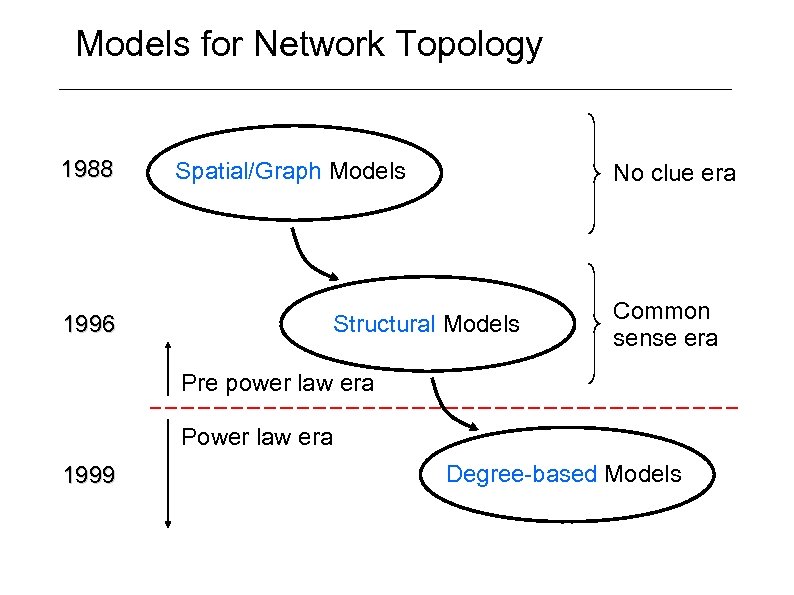Models for Network Topology 1988 Spatial/Graph Models No clue era Structural Models 1996 Common sense era Pre power law era Power law era 1999 Degree-based Models

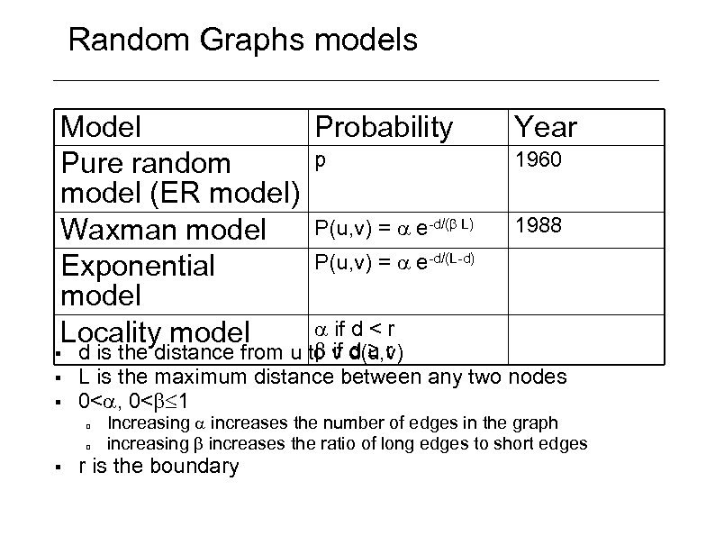Random Graphs models Model Probability p Pure random model (ER model) P(u, v) = e-d/( L) Waxman model P(u, v) = e-d/(L-d) Exponential model if d < r Locality model § § § 1960 1988 if d ≥ r d is the distance from u to v d(u, v) L is the maximum distance between any two nodes 0< , 0< 1 § Year Increasing increases the number of edges in the graph increasing increases the ratio of long edges to short edges r is the boundary

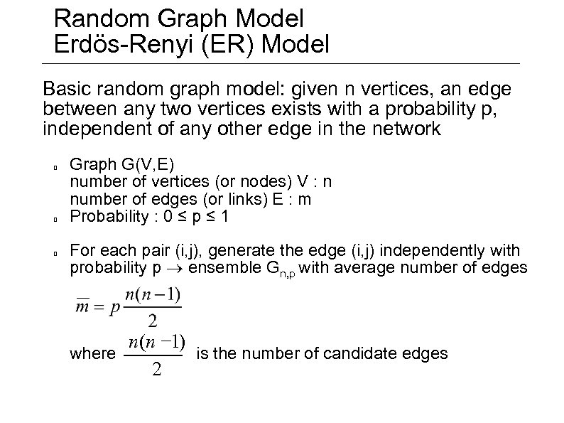Random Graph Model Erdös-Renyi (ER) Model Basic random graph model: given n vertices, an edge between any two vertices exists with a probability p, independent of any other edge in the network Graph G(V, E) number of vertices (or nodes) V : n number of edges (or links) E : m Probability : 0 ≤ p ≤ 1 For each pair (i, j), generate the edge (i, j) independently with probability p ensemble Gn, p with average number of edges n(n -1) where is the number of candidate edges 2

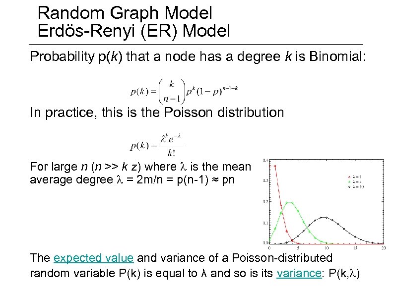Random Graph Model Erdös-Renyi (ER) Model Probability p(k) that a node has a degree k is Binomial: In practice, this is the Poisson distribution For large n (n >> k z) where is the mean average degree = 2 m/n = p(n-1) ≈ pn The expected value and variance of a Poisson-distributed random variable P(k) is equal to λ and so is its variance: P(k, )

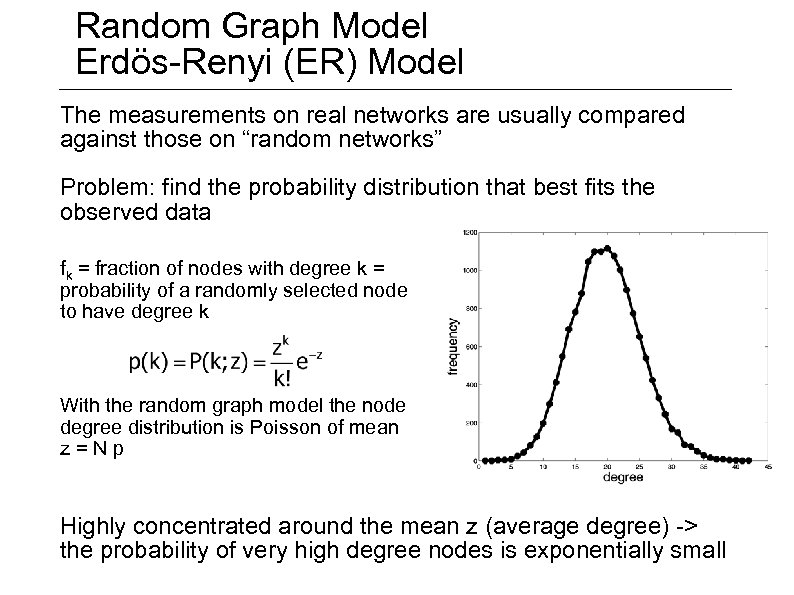Random Graph Model Erdös-Renyi (ER) Model The measurements on real networks are usually compared against those on “random networks” Problem: find the probability distribution that best fits the observed data fk = fraction of nodes with degree k = probability of a randomly selected node to have degree k With the random graph model the node degree distribution is Poisson of mean z=Np Highly concentrated around the mean z (average degree) -> the probability of very high degree nodes is exponentially small

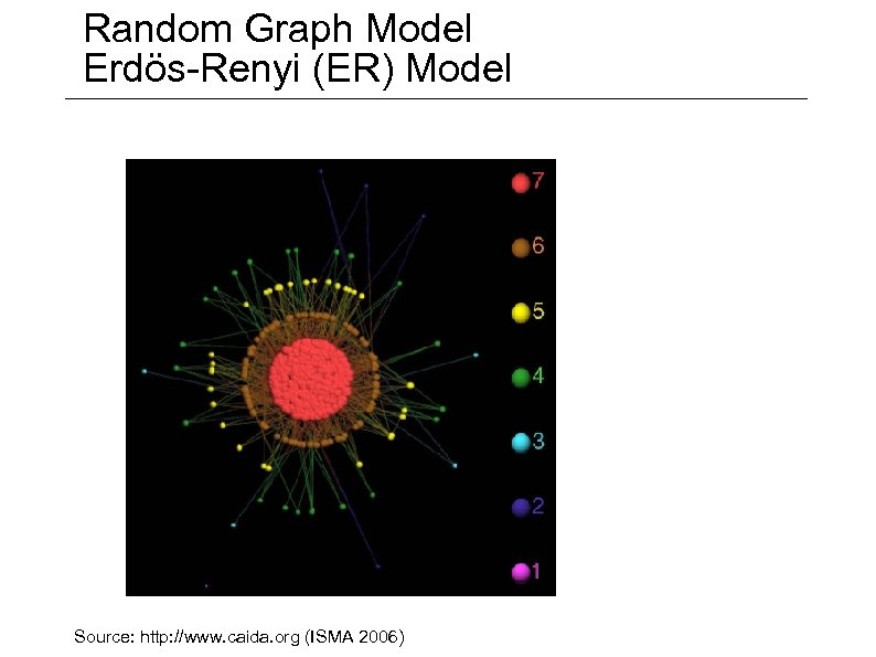Random Graph Model Erdös-Renyi (ER) Model Source: http: //www. caida. org (ISMA 2006)

Waxman Models and Generators (Waxman 1988) Waxman model: Router-level model capturing locality Idea based on the observation that long-range links are expensive – – Variant of random graphs (ER model) where the probability that any two vertices are connected decreases with the increasing distance between them Intuitively: the farther apart the two nodes are, the less likely they will be connected) Successful only in representing small networks

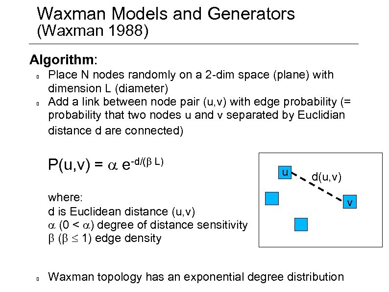Waxman Models and Generators (Waxman 1988) Algorithm: Place N nodes randomly on a 2 -dim space (plane) with dimension L (diameter) Add a link between node pair (u, v) with edge probability (= probability that two nodes u and v separated by Euclidian distance d are connected) P(u, v) = e-d/( L) u d(u, v) where: d is Euclidean distance (u, v) (0 < ) degree of distance sensitivity ( 1) edge density Waxman topology has an exponential degree distribution v

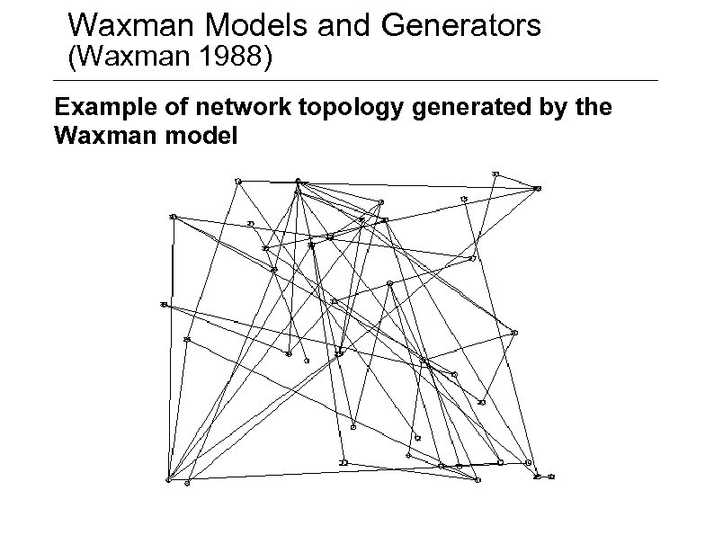Waxman Models and Generators (Waxman 1988) Example of network topology generated by the Waxman model

Random Graph Model Erdös-Renyi (ER) Model Are E-R graphs realistic? § They have small world properties (diameter is logarithmic in the size of the graph) but low clustering coefficient: Example for autonomous internet systems, compare 0. 30 with 0. 0004 [Pastor-Satorras and Vespignani] § Unrealistic degree distributions: degrees not concentrated around mean § Exponential tails: instead heavy tailed degree distribution § Result: departure from ER model and variants

Outline 1. Organization of the Internet 2. Evolution of the Internet 3. Internet Topology modelling Network properties Random Graphs models and generators Structural models and generators Topology measurements Power Law relationships Degree-based models and generators Internet topology metrics

Structural Models Based on the observation that real networks are not structured randomly (engineering dimension) but exhibit Hierarchical structure (two or three tier-level structure) Specialized domains (transit domains, stub domains) Connectivity requirements Redundancy (resiliency) Characteristics incorporated into Tiers generator GT-ITM: Georgia Tech Internetwork Topology Models

Structural Generators: Tiers (Doar 1996) § Router level model capturing hierarchy § Three level hierarchy model (3 -level Tiers) comprising LAN, MAN, and WAN Can specify numbers of LAN, and MAN partitions, number of WANs = 1 (connected) LANs are modeled as star with router at center and host around (star-shaped LANs) Produces connected sub-graphs by joining all nodes in one domain using a spanning tree: WAN and MANs are first connected using a spanning tree (guarantees connectivity) Remaining links connected in order of increasing distance Closer connections preferred, like a mesh/grid Adding edges for intra-domain and inter-domain redundancy

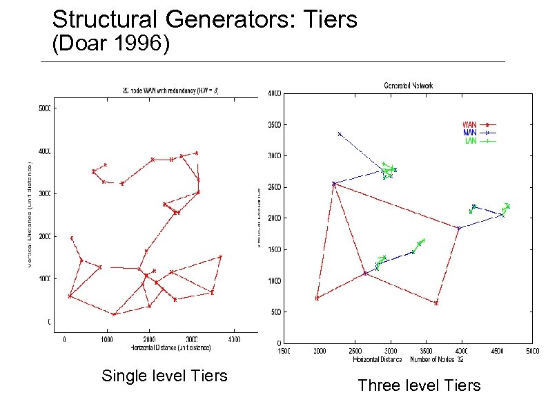Structural Generators: Tiers (Doar 1996) Single level Tiers Three level Tiers

Structural Generators: Transit-Stub (Calvert/Zegura 1997) § Router level model capturing hierarchy § Basic idea § Combination of number of simple topologies in a hierarchical structure: transit domains and stub domains modelled as random graphs Supports only two-level hierarchy Transit-Stub generator Generate a connected random graph where each node is replace by connected random graph (transit domain) For each node in transit domain, a number of connected random graphs (stub domains) are generated and attached to that transit node by transit-stub links Add some “extra” connectivity: transit-stub links, and stub-stub links Possibility to assign edge weights Several user-specified parameters to control the structure of the graph: N transit domains and M stub domains with n and m average routers, ratio stub to transit ( need for experimental estimates to set values to the parameters of the model)

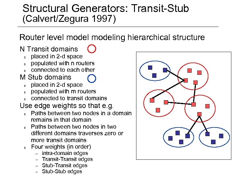Structural Generators: Transit-Stub (Calvert/Zegura 1997) Router level modeling hierarchical structure N Transit domains placed in 2 -d space populated with n routers connected to each other M Stub domains placed in 2 -d space populated with m routers connected to transit domains Use edge weights so that e. g. Paths between two nodes in a domain remains in that domain Paths between two nodes in two different domains traverses zero or more transit domains Four weights (in order) – – intra-domain edges Transit-Transit edges Stub-Stub edges

Structural Generators: Transit-Stub GT-ITM GT‐ITM (Georgia Tech Internetwork Topology Models) Router-level model simulator capturing the actual Internet hierarchy by differentiating structural elements: the transit and the stub domains Transit domain Number of transit domains placed in 2 -dim space Populated with routers and connected to each other Stub domain Number of stub domains placed in 2 -dim space Populated with routers Connected to transit domains Transit-stub Connectivity

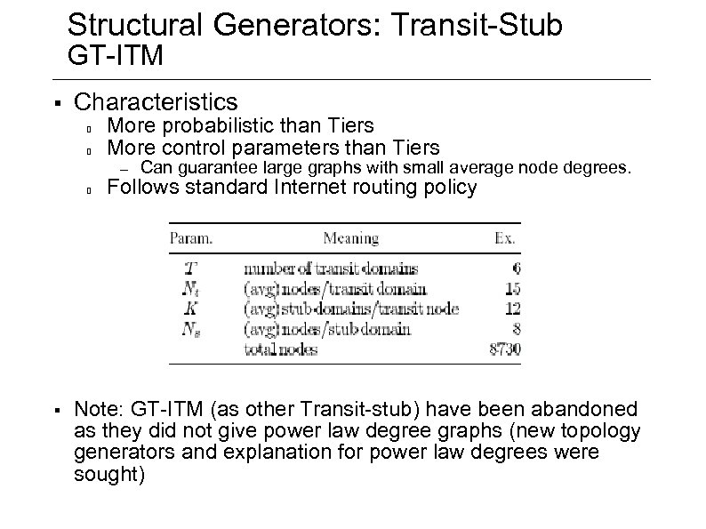Structural Generators: Transit-Stub GT-ITM § Characteristics More probabilistic than Tiers More control parameters than Tiers – § Can guarantee large graphs with small average node degrees. Follows standard Internet routing policy Note: GT-ITM (as other Transit-stub) have been abandoned as they did not give power law degree graphs (new topology generators and explanation for power law degrees were sought)

Outline 1. Organization of the Internet 2. Evolution of the Internet 3. Internet Topology modelling Network properties Random Graphs models and generators Structural models and generators Topology measurements Power Law relationships Degree-based models and generators Internet topology metrics

Topology measurement 1. Router-level topologies reflect physical connectivity between nodes Inferred from tools like traceroute or well known public measurement projects like Mercator and Skitter 2. AS-level Internet topology where AS graph reflects a peering relationship between two providers/clients Inferred from inter-domain routers that run BGP and public projects like Oregon Route Views

Topology measurement Router-level Internet topology § Construction Probing techniques (e. g. traceroute) discovers compliant IP routers along path between selected network host computers Coupled with source-routing (requires sourcerouting enabled routers, which are only about 8% of the total routers) and removing aliases (which IP addresses belong to same router) Interface collapsing algorithms

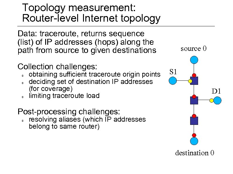Topology measurement: Router-level Internet topology Data: traceroute, returns sequence (list) of IP addresses (hops) along the path from source to given destinations Collection challenges: obtaining sufficient traceroute origin points deciding set of destination IP addresses (for coverage) limiting traceroute load source 0 S 1 D 1 Post-processing challenges: resolving aliases (which IP addresses belong to same router) destination 0

Topology measurement: Router-level Internet topology § Examples of Large-scale traceroute experiments Pansiot and Grad: router-level map from around 1995 Cheswick and Burch: mapping project started in 1997 Mercator (single source with source-routing): router-level maps from around 1999 by R. Govindan and H. Tangmunarunkit) CAIDA Skitter: multiple sources (now replaced by “Archipelagos measurement infrastructure” or Ark (*) – – Traceroute based tool Continuous measurement since 1998 25 monitors distributed over the Internet Monitor destination list of 1 million IPv 4 addresses Rocketfuel: router-level maps of individual ISPs by Univ. of Washington (http: //www. cs. washington. edu/research/networking/rocketfuel/) Dimes (EU project) (*) http: //www. caida. org/publications/presentations/2006/young_wide 0611_ark. pdf

Problems with Traceroute-based measurements § Ambiguity § Inaccuracy § traceroute is strictly about IP-level connectivity traceroute cannot distinguish between high connectivity nodes that are for real and that are fake and due to underlying Layer 2 (e. g. , Ethernet, ATM) or MPLS Requires some guesswork in deciding which IP addresses/interface cards refer to the same router (“alias resolution” problem) Incomplete/biased IP-level connectivity is more easily/accurately inferred the closer the routers are to the traceroute source(s) Node degree distribution is inferred to be of the power-law type even when the actual distribution is not

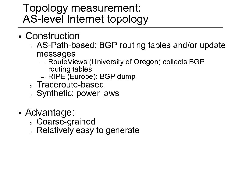Topology measurement: AS-level Internet topology § Construction AS-Path-based: BGP routing tables and/or update messages – – § Route. Views (University of Oregon) collects BGP routing tables RIPE (Europe): BGP dump Traceroute-based Synthetic: power laws Advantage: Coarse-grained Relatively easy to generate

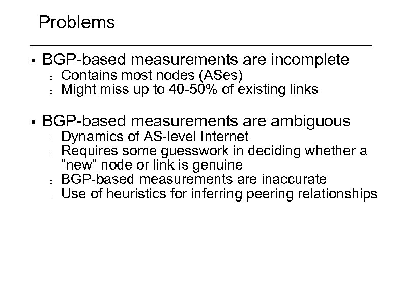Problems § BGP-based measurements are incomplete § Contains most nodes (ASes) Might miss up to 40 -50% of existing links BGP-based measurements are ambiguous Dynamics of AS-level Internet Requires some guesswork in deciding whether a “new” node or link is genuine BGP-based measurements are inaccurate Use of heuristics for inferring peering relationships

Outline 1. Organization of the Internet 2. Evolution of the Internet 3. Internet Topology modelling Network properties Random Graphs models and generators Structural models and generators Topology measurements Power Law relationships Degree-based models and generators Internet topology metrics

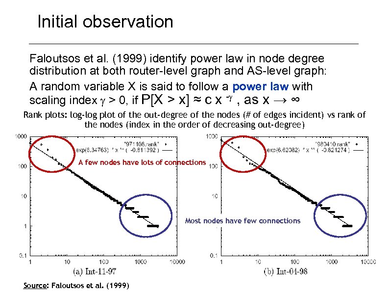Initial observation Faloutsos et al. (1999) identify power law in node degree distribution at both router-level graph and AS-level graph: A random variable X is said to follow a power law with scaling index g > 0, if P[X > x] ≈ c x -g , as x → ∞ Rank plots: log-log plot of the out-degree of the nodes (# of edges incident) vs rank of the nodes (index in the order of decreasing out-degree) A few nodes have lots of connections Most nodes have few connections Source: Faloutsos et al. (1999)

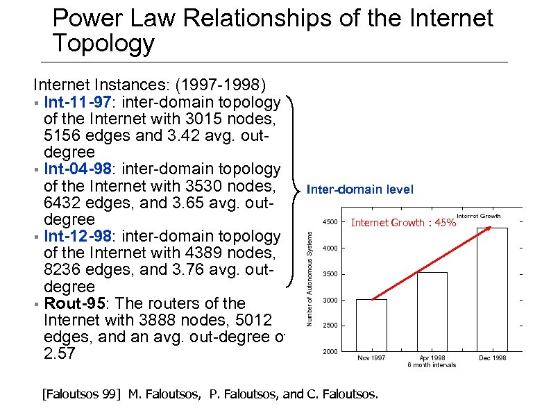Power Law Relationships of the Internet Topology Internet Instances: (1997 -1998) § Int-11 -97: inter-domain topology of the Internet with 3015 nodes, 5156 edges and 3. 42 avg. outdegree § Int-04 -98: inter-domain topology of the Internet with 3530 nodes, 6432 edges, and 3. 65 avg. outdegree § Int-12 -98: inter-domain topology of the Internet with 4389 nodes, 8236 edges, and 3. 76 avg. outdegree § Rout-95: The routers of the Internet with 3888 nodes, 5012 edges, and an avg. out-degree of 2. 57 Inter-domain level Internet Growth : 45% [Faloutsos 99] M. Faloutsos, P. Faloutsos, and C. Faloutsos.

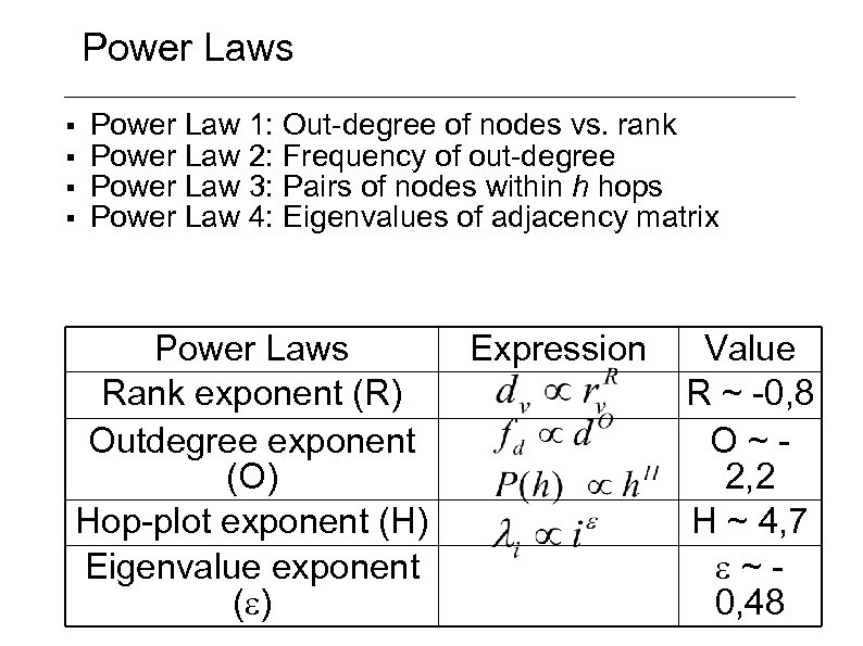Power Laws § § Power Law 1: Out-degree of nodes vs. rank Power Law 2: Frequency of out-degree Power Law 3: Pairs of nodes within h hops Power Law 4: Eigenvalues of adjacency matrix Power Laws Rank exponent (R) Outdegree exponent (O) Hop-plot exponent (H) Eigenvalue exponent ( ) Expression Value R ~ -0, 8 O~2, 2 H ~ 4, 7 ~0, 48

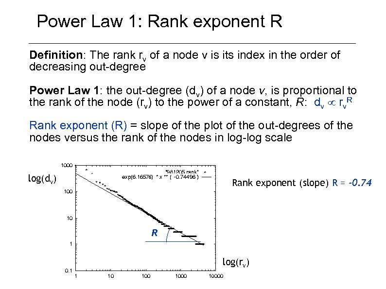Power Law 1: Rank exponent R Definition: The rank rv of a node v is its index in the order of decreasing out-degree Power Law 1: the out-degree (dv) of a node v, is proportional to the rank of the node (rv) to the power of a constant, R: dv rv. R Rank exponent (R) = slope of the plot of the out-degrees of the nodes versus the rank of the nodes in log-log scale log(dv) Rank exponent (slope) R = -0. 74 R log(rv)

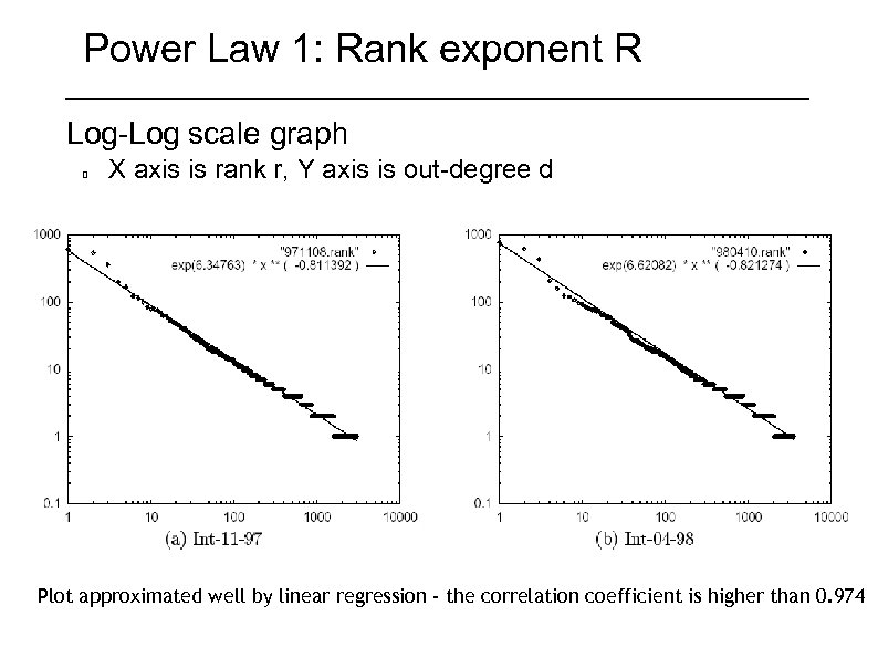Power Law 1: Rank exponent R Log-Log scale graph X axis is rank r, Y axis is out-degree d Plot approximated well by linear regression - the correlation coefficient is higher than 0. 974 !

Power Law 1: Rank exponent R Observations: For the 3 interdomain-level instances, the rank exponent is 0. 81, -0. 82 and -0. 74 For the router-level graph, the rank exponent is -0. 48 This difference suggests that the rank exponent can distinguish graphs of different nature (e. g. inter-domain vs. intra-domain) Interpretation: This power-law most likely reflects a principle of the way domains and routers connect Captures equilibrium of the trade-off between the gain and the cost of adding an edge from a financial and functional point of view

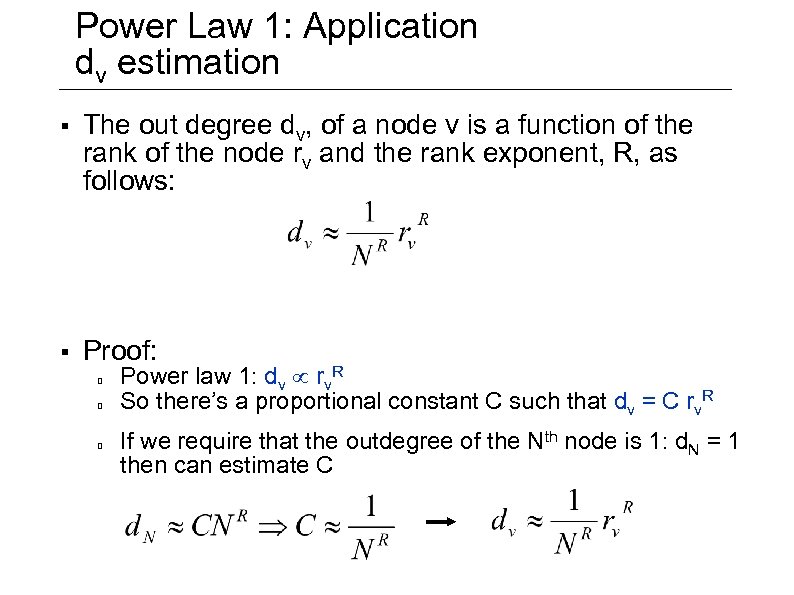Power Law 1: Application dv estimation § The out degree dv, of a node v is a function of the rank of the node rv and the rank exponent, R, as follows: § Proof: Power law 1: dv rv. R So there’s a proportional constant C such that dv = C rv. R If we require that the outdegree of the Nth node is 1: d. N = 1 then can estimate C

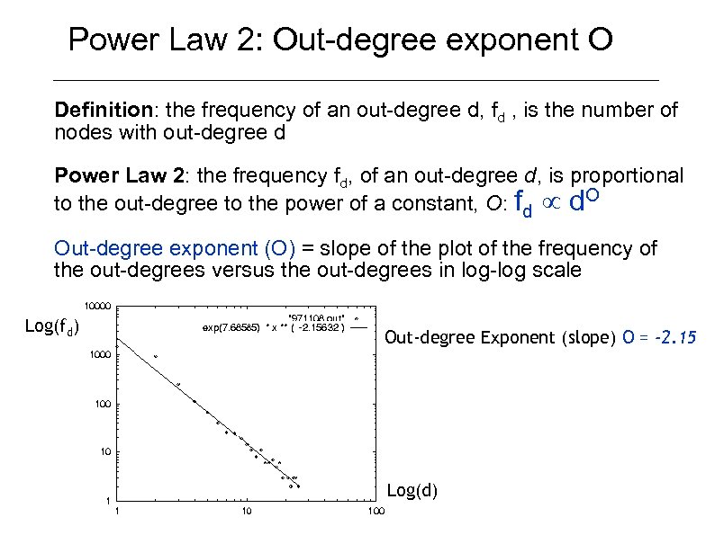Power Law 2: Out-degree exponent O Definition: the frequency of an out-degree d, fd , is the number of nodes with out-degree d Power Law 2: the frequency fd, of an out-degree d, is proportional to the out-degree to the power of a constant, O: fd d. O Out-degree exponent (O) = slope of the plot of the frequency of the out-degrees versus the out-degrees in log-log scale Log(fd) Out-degree Exponent (slope) O = -2. 15 Log(d)

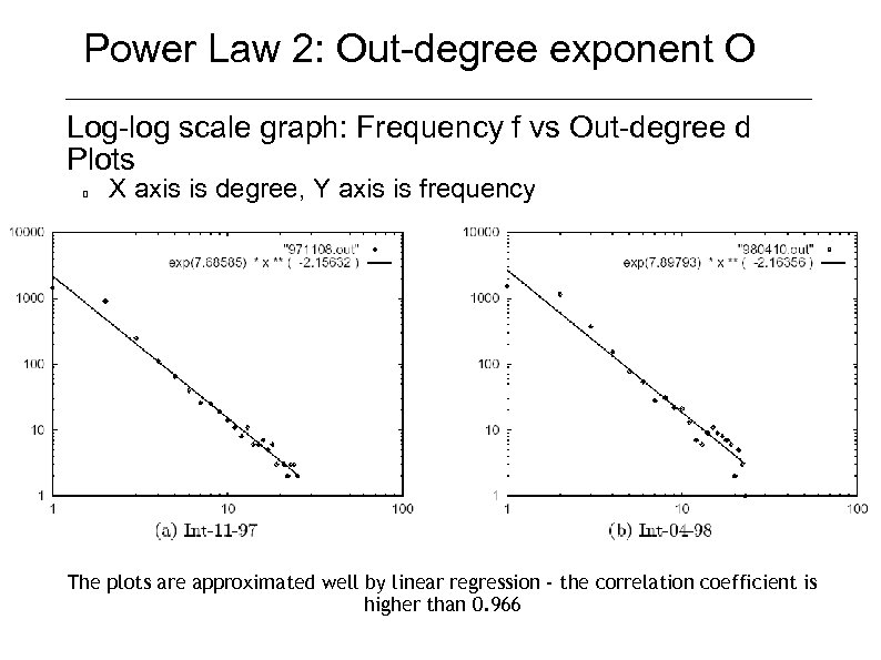Power Law 2: Out-degree exponent O Log-log scale graph: Frequency f vs Out-degree d Plots X axis is degree, Y axis is frequency The plots are approximated well by linear regression - the correlation coefficient is higher than 0. 966

Power Law 2: Out-degree exponent O Observation The value of the out-degree exponent is practically constant For the inter-domain topology, the out-degree exponent O is: -2. 15, -2. 16 and -2. 2 For the router-level, the out-degree exponent O router-level topology is -2. 48 Interpretation Suggest that the out-degree exponent O describes a fundamental property of the network: lower degrees are more frequent

Power Law 3: Hop-Plot Exponent H Definition: the neighborhood size P(h) of distance h, is the total number of pairs of nodes within less or equal to h hops, including self-pairs, and counting all other pairs twice Examples For h = 0, only self-pairs: P(0) = N For h = δ (graph diameter) self-pairs and all other possible pairs: P(δ) = N 2 (maximum possible number of pairs) Idea For a ring topology we have P(h) h 1 For a 2 -dimensional grid, we have P(h) h 2 (for h « δ) Question: Will the number of pairs P(h) for the Internet follows a similar power-law ?

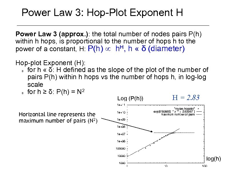Power Law 3: Hop-Plot Exponent H Power Law 3 (approx. ): the total number of nodes pairs P(h) within h hops, is proportional to the number of hops h to the power of a constant, H: P(h) h. H, h « δ (diameter) Hop-plot Exponent (H): for h « δ: H defined as the slope of the plot of the number of pairs P(h) within h hops vs the number of hops h, in log-log scale for h ≥ δ: P(h) = N 2 Log (P(h)) H = 2. 83 Horizontal line represents the maximum number of pairs (N 2) log(h)

Power Law 3: Hop-Plot Exponent H § Observation § The 3 domain-level datasets have practically equal hopplot exponents: H ~ 4, 7 The router-level dataset has a hop-plot H exponent of 2, 8 Interpretation The hop-plot exponent can distinguish families of graphs efficiently

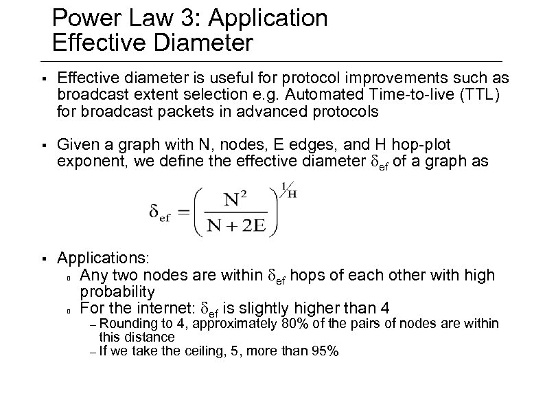Power Law 3: Application Effective Diameter § Effective diameter is useful for protocol improvements such as broadcast extent selection e. g. Automated Time-to-live (TTL) for broadcast packets in advanced protocols § Given a graph with N, nodes, E edges, and H hop-plot exponent, we define the effective diameter def of a graph as § Applications: Any two nodes are within def hops of each other with high probability For the internet: def is slightly higher than 4 – Rounding to 4, approximately 80% of the pairs of nodes are within this distance – If we take the ceiling, 5, more than 95%

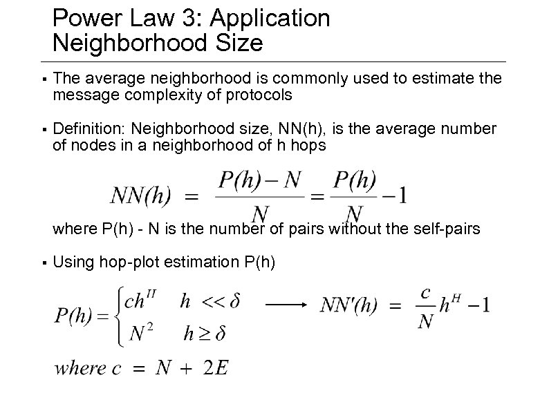Power Law 3: Application Neighborhood Size § The average neighborhood is commonly used to estimate the message complexity of protocols § Definition: Neighborhood size, NN(h), is the average number of nodes in a neighborhood of h hops where P(h) - N is the number of pairs without the self-pairs § Using hop-plot estimation P(h)

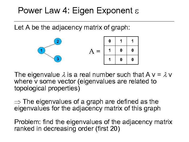Power Law 4: Eigen Exponent Let A be the adjacency matrix of graph: 0 2 A= 1 3 1 1 1 0 0 The eigenvalue l is a real number such that A v = l v where v some vector (eigenvalues are related to topological properties) The eigenvalues of a graph are defined as the eigenvalues for the adjacency matrix of this graph Problem: find the eigenvalues of the adjacency matrix ranked in decreasing order (first 20)

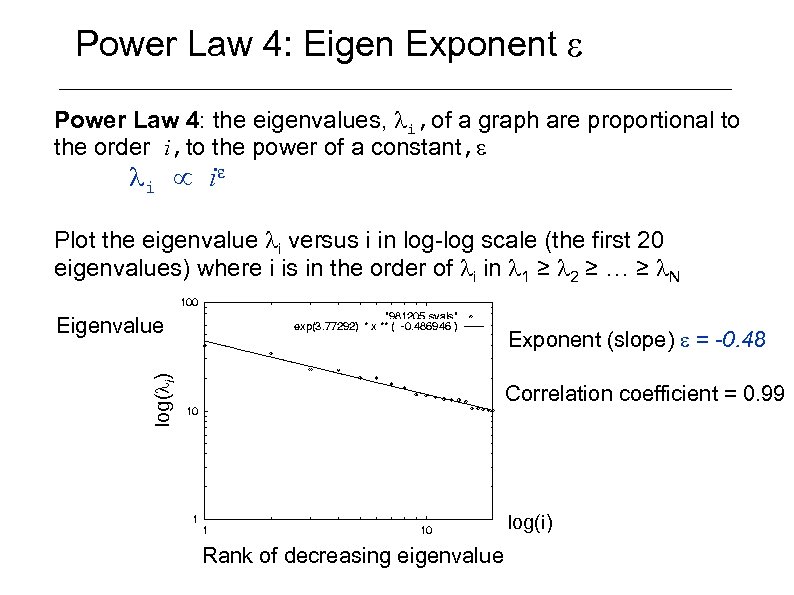Power Law 4: Eigen Exponent Power Law 4: the eigenvalues, i, of a graph are proportional to the order i, to the power of a constant, i i Plot the eigenvalue i versus i in log-log scale (the first 20 eigenvalues) where i is in the order of i in 1 ≥ 2 ≥ … ≥ N Eigenvalue log( i) Exponent (slope) = -0. 48 Correlation coefficient = 0. 99 log(i) Rank of decreasing eigenvalue

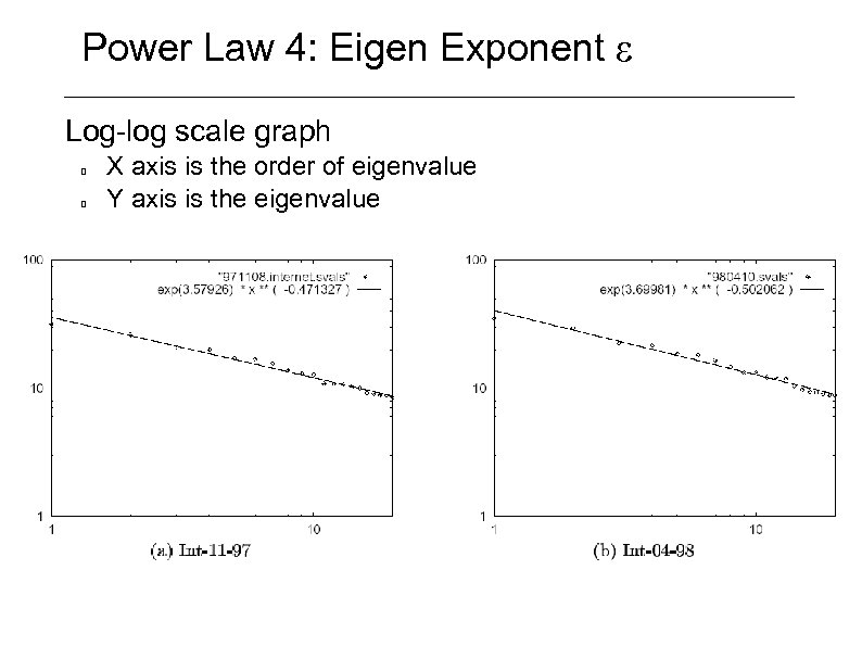Power Law 4: Eigen Exponent Log-log scale graph X axis is the order of eigenvalue Y axis is the eigenvalue

Power Law 4: Eigen Exponent § Eigen exponents value for the interdomain-level graphs: ~ -0, 48 for the router-level graph: = -, 0177 can also distinguish families of graphs efficiently § Rich literature proves that eigenvalues of a graph are closely related to topological properties of graphs Graph diameter, number of edges, number of spanning trees Number of connected components, and more

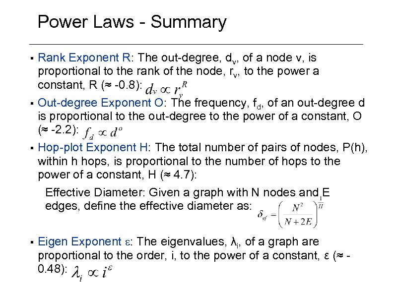Power Laws - Summary Rank Exponent R: The out-degree, dv, of a node v, is proportional to the rank of the node, rv, to the power a constant, R (≈ -0. 8): § Out-degree Exponent O: The frequency, fd, of an out-degree d is proportional to the out-degree to the power of a constant, O (≈ -2. 2): § Hop-plot Exponent H: The total number of pairs of nodes, P(h), within h hops, is proportional to the number of hops to the power of a constant, H (≈ 4. 7): Effective Diameter: Given a graph with N nodes and E edges, define the effective diameter as: § § Eigen Exponent : The eigenvalues, λi, of a graph are proportional to the order, i, to the power of a constant, ε (≈ 0. 48):

Outline 1. Organization of the Internet 2. Evolution of the Internet 3. Internet Topology modelling Network properties Random Graphs models and generators Structural models and generators Topology measurements Power Law relationships Degree-based models and generators Internet topology metrics

Degree-based Network Topology Models § Faloutsos et al. (1999) find power law in node degree distribution at router-level graph & Autonomous System (AS) graph § Basic Idea: traditional random graphs [Erdös & Renyí, 1959] do not produce power laws, so develop new models that explicitly attempt to match the observed (power law) distribution in node degree Led to active research in degree-based network models: focus on generators that match degree distribution of observed graph (descriptive methods)

Degree-based Network Topology Generators § Two methods for generating random networks having power law distributions in node degree Growth modelling (evolutionary) – – – Distribution modelling (non-evolutionary) – § Inet 3. 0: enforced power law degree distribution and Preferential Attachment BRITE: model based on Incremental growth and Preferential Attachment Barabasi-Albert (BA) model: scale free networks characterized by Incremental growth and Preferential Attachment Albert-Barabasi (AB) model: variant of BA model Generalized Linear Preference (GLP) model Expected Degree Sequence (Given Expected Degree): Power Law Random Graph (PLRG) and Generalized Random Graph (GRG) Common features: Ignore all system-specific details Central core of high-degree, hub-like nodes

Inet model (Jin 2000) § AS level Internet topology generator § Number of links generated depends on § Originally designed to match the measurements of the original-maps of the AS graph Total number of nodes Percentage of nodes with degree 1 Typically generates 26% less links than extended-AS graph

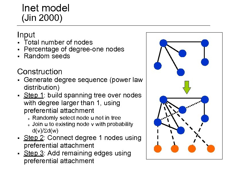Inet model (Jin 2000) Input § § § Total number of nodes Percentage of degree-one nodes Random seeds Construction § § Generate degree sequence (power law distribution) Step 1: build spanning tree over nodes with degree larger than 1, using preferential attachment § § Randomly select node u not in tree Join u to existing node v with probability d(v)/ d(w) Step 2: Connect degree 1 nodes using preferential attachment Step 3: Add remaining edges using preferential attachment

BRITE (Medina 2000) § Capture properties § Key Ideas § Power law relationship Network evolution (incremental growth) Preferential attachment of a new node to existing nodes Incremental growth of the network Connection locality Input Size of plane (to assign the node) Number of links added per new node Incremental growth Preferential attachment

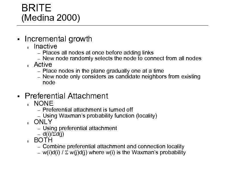BRITE (Medina 2000) § Incremental growth Inactive – – § Places all nodes at once before adding links New node randomly selects the node to connect from all nodes Place nodes in the plane gradually one at a time New node only considers as candidate neighbors from existing node Active Preferential Attachment NONE – – Preferential attachment is turned off Using Waxman’s probability function (locality) Using preferential attachment d(i)/ d(j) – – Combine preferential attachment and connection locality w(i)d(i) / w(j)d(j) where w(i) is the Waxman’s probability ONLY BOTH

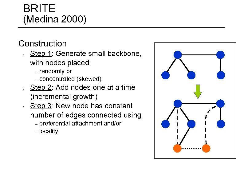BRITE (Medina 2000) Construction Step 1: Generate small backbone, with nodes placed: – – randomly or concentrated (skewed) Step 2: Add nodes one at a time (incremental growth) Step 3: New node has constant number of edges connected using: – – preferential attachment and/or locality

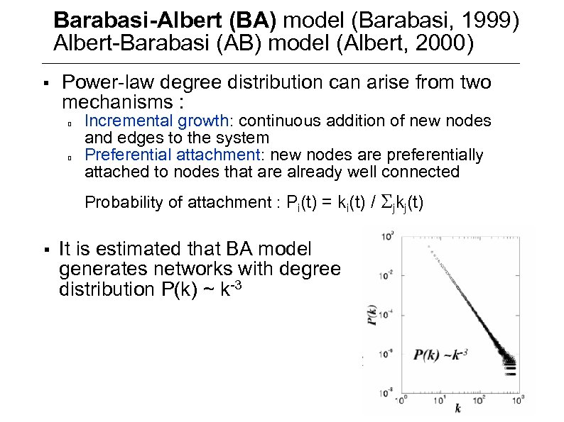Barabasi-Albert (BA) model (Barabasi, 1999) Albert-Barabasi (AB) model (Albert, 2000) § Power-law degree distribution can arise from two mechanisms : Incremental growth: continuous addition of new nodes and edges to the system Preferential attachment: new nodes are preferentially attached to nodes that are already well connected Probability of attachment : Pi(t) = ki(t) / jkj(t) § It is estimated that BA model generates networks with degree distribution P(k) ~ k-3

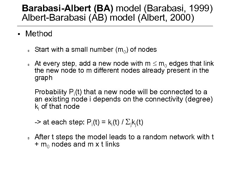Barabasi-Albert (BA) model (Barabasi, 1999) Albert-Barabasi (AB) model (Albert, 2000) § Method Start with a small number (m 0) of nodes At every step, add a new node with m m 0 edges that link the new node to m different nodes already present in the graph Probability Pi(t) that a new node will be connected to a an existing node i depends on the connectivity (degree) ki of that node -> at each step: Pi(t) = ki(t) / jkj(t) After t steps the model leads to a random network with t + m 0 nodes and m x t links

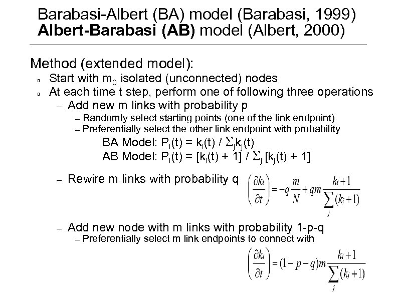Barabasi-Albert (BA) model (Barabasi, 1999) Albert-Barabasi (AB) model (Albert, 2000) Method (extended model): Start with m 0 isolated (unconnected) nodes At each time t step, perform one of following three operations – Add new m links with probability p – – Randomly select starting points (one of the link endpoint) Preferentially select the other link endpoint with probability BA Model: Pi(t) = ki(t) / jkj(t) AB Model: Pi(t) = [ki(t) + 1] / j [kj(t) + 1] – Rewire m links with probability q – Add new node with m links with probability 1 -p-q – Preferentially select m link endpoints to connect with

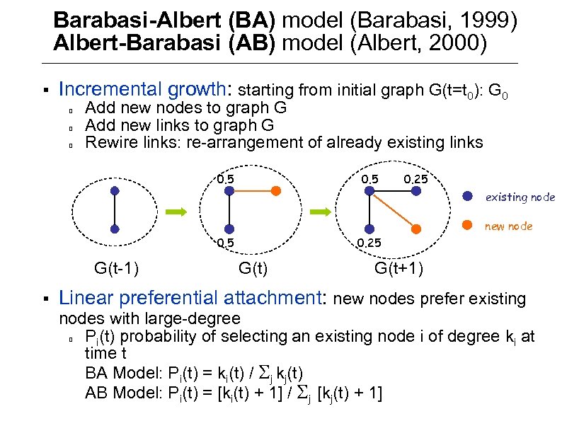Barabasi-Albert (BA) model (Barabasi, 1999) Albert-Barabasi (AB) model (Albert, 2000) § Incremental growth: starting from initial graph G(t=t 0): G 0 Add new nodes to graph G Add new links to graph G Rewire links: re-arrangement of already existing links 0. 5 0. 25 existing node new node 0. 5 G(t-1) § 0. 25 G(t) G(t+1) Linear preferential attachment: new nodes prefer existing nodes with large-degree Pi(t) probability of selecting an existing node i of degree ki at time t BA Model: Pi(t) = ki(t) / j kj(t) AB Model: Pi(t) = [ki(t) + 1] / j [kj(t) + 1]

Generalized Linear Preference (GLP) (Bu, 2002) § § A modification of the BA model Evolution of AS graph mostly due to two reasons § Addition of new nodes Addition of new links between existing nodes Method It starts with m 0 nodes connected through m 0 -1 links At each time step (t), perform one of the following two operations: – – With probability p, add m < m 0 new links between m pairs of nodes chosen from existing nodes (for each end of each link, node i is chosen with probability Pi(t) With probability 1 -p, add new node with m new links and connected to m existing nodes (each link is connected to node i already present in the system with probability Pi(t) Growth of new nodes and new links are independent (the probability that node i increases its degree ki is a function of that degree)

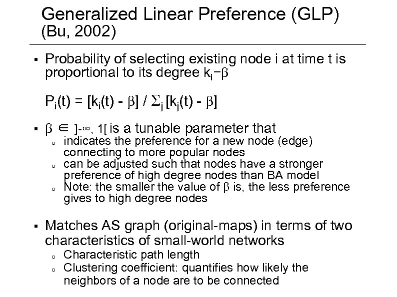Generalized Linear Preference (GLP) (Bu, 2002) § Probability of selecting existing node i at time t is proportional to its degree ki− Pi(t) = [ki(t) - ] / j [kj(t) - ] § ∈ ]-∞, 1[ is a tunable parameter that § indicates the preference for a new node (edge) connecting to more popular nodes can be adjusted such that nodes have a stronger preference of high degree nodes than BA model Note: the smaller the value of is, the less preference gives to high degree nodes Matches AS graph (original-maps) in terms of two characteristics of small-world networks Characteristic path length Clustering coefficient: quantifies how likely the neighbors of a node are to be connected

Expected Degree Sequence § Non-evolutionary models § Based on random graph models (inspired by graph theory) that skew probability distribution to produce power laws in expectation (expected degree sequence) § Examples: Power Law Random Graph (PLRG) [Aiello 00]: enforce power law degree distribution and random matching of nodes Generalized Random Graph (GRG) [Chung 03]

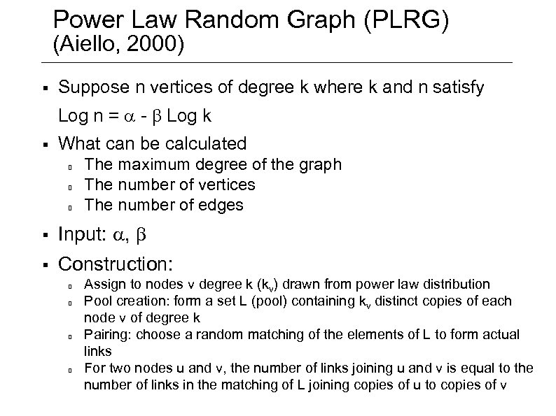Power Law Random Graph (PLRG) (Aiello, 2000) § Suppose n vertices of degree k where k and n satisfy Log n = - Log k § What can be calculated The maximum degree of the graph The number of vertices The number of edges § Input: , § Construction: Assign to nodes v degree k (kv) drawn from power law distribution Pool creation: form a set L (pool) containing kv distinct copies of each node v of degree k Pairing: choose a random matching of the elements of L to form actual links For two nodes u and v, the number of links joining u and v is equal to the number of links in the matching of L joining copies of u to copies of v

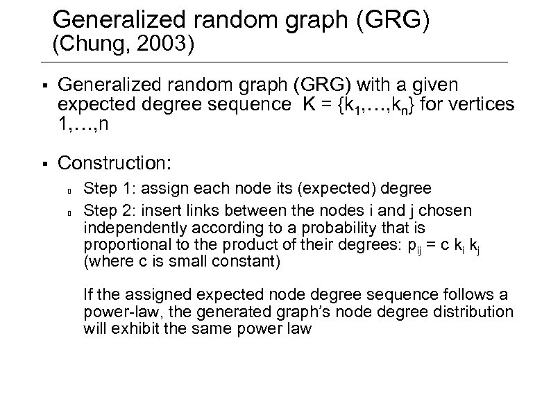Generalized random graph (GRG) (Chung, 2003) § Generalized random graph (GRG) with a given expected degree sequence K = {k 1, …, kn} for vertices 1, …, n § Construction: Step 1: assign each node its (expected) degree Step 2: insert links between the nodes i and j chosen independently according to a probability that is proportional to the product of their degrees: pij = c ki kj (where c is small constant) If the assigned expected node degree sequence follows a power-law, the generated graph’s node degree distribution will exhibit the same power law

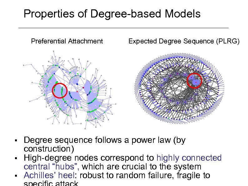Properties of Degree-based Models Preferential Attachment § § § Expected Degree Sequence (PLRG) Degree sequence follows a power law (by construction) High-degree nodes correspond to highly connected central “hubs”, which are crucial to the system Achilles’ heel: robust to random failure, fragile to

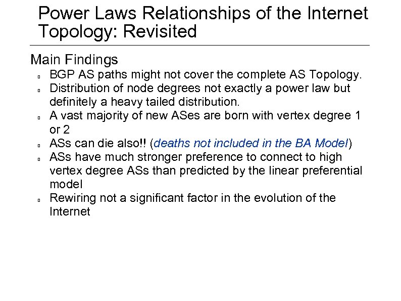Power Laws Relationships of the Internet Topology: Revisited Main Findings BGP AS paths might not cover the complete AS Topology. Distribution of node degrees not exactly a power law but definitely a heavy tailed distribution. A vast majority of new ASes are born with vertex degree 1 or 2 ASs can die also!! (deaths not included in the BA Model) ASs have much stronger preference to connect to high vertex degree ASs than predicted by the linear preferential model Rewiring not a significant factor in the evolution of the Internet

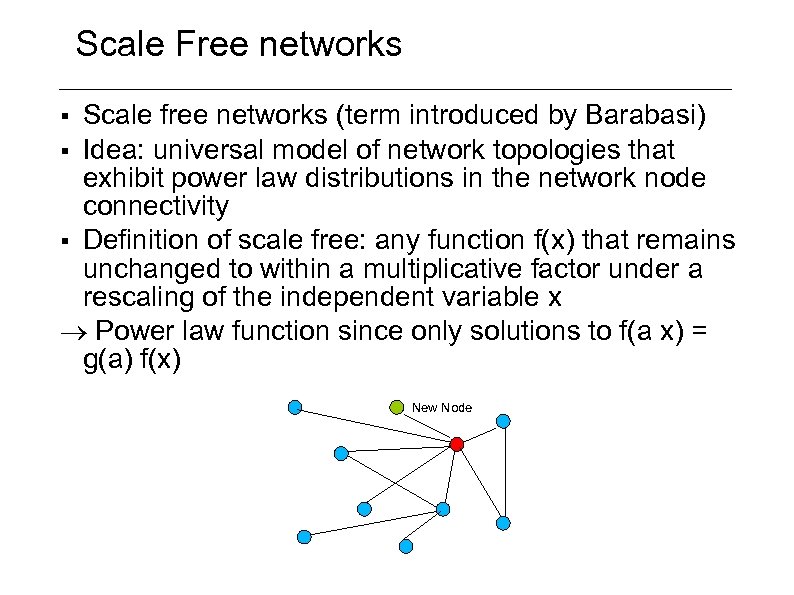Scale Free networks Scale free networks (term introduced by Barabasi) § Idea: universal model of network topologies that exhibit power law distributions in the network node connectivity § Definition of scale free: any function f(x) that remains unchanged to within a multiplicative factor under a rescaling of the independent variable x Power law function since only solutions to f(a x) = g(a) f(x) § New Node

Scale Free networks 1. Continuous (incremental) growth Existing models of networks did not include the addition of nodes over time. The graphs remained static. Scale free networks are in a state of continuous growth by incremental addition of new nodes and links to the system 2. Preferential attachment New nodes tend to connect to nodes that are already well connected. New nodes have higher probability of connecting to the existing nodes with high connectivity, i. e. , a “rich-gets-richer” “Rich club” phenomenon - power laws in asymptotic limit: new nodes attach preferentially to high-degree nodes (well -connected nodes) in linear proportion to their degree Note: Role of Rewiring process: Re-arrangement of the already existing links

Rich Club Phenomenon Rich nodes Power-law technologies have small number of nodes having large number of links AS graph shows this phenomenon Rich nodes are well connected to each other Rich nodes are connected preferentially to the other rich nodes Measured in the Original-maps of the AS graph (BGP Routing tables by University of Oregon Route Views Project) Extended-maps of the AS graph (BGP Routing tables + Looking Glass (LG) data + Internet Routing Registry data)

Scale Free networks - Controversy Scientists spot Achilles heel of the Internet Fact: scale-free networks have approximately power law degree distributions Claim: If the Internet has power law degree distribution Then, the Internet must be scale-free ⇒ The Internet has the properties of a scale-free network Implications of “scale free” network structure Few centrally located and highly connected hubs (highdegree nodes correspond to highly connected central “hubs”, critical to the system) ⇒ Achilles’ heel: robust to random attack/node failures (probability of targeting hub very low) but vulnerable to targeted attacks "The reason this is so is because there a couple of very big nodes and all messages are going through them. But if someone maliciously takes down the biggest nodes you can harm the system in incredible ways. You can very easily destroy the function of the Internet, . . . " -- “Achilles heel of the Internet” Albert, Jeong, Barabasi, Nature 2000

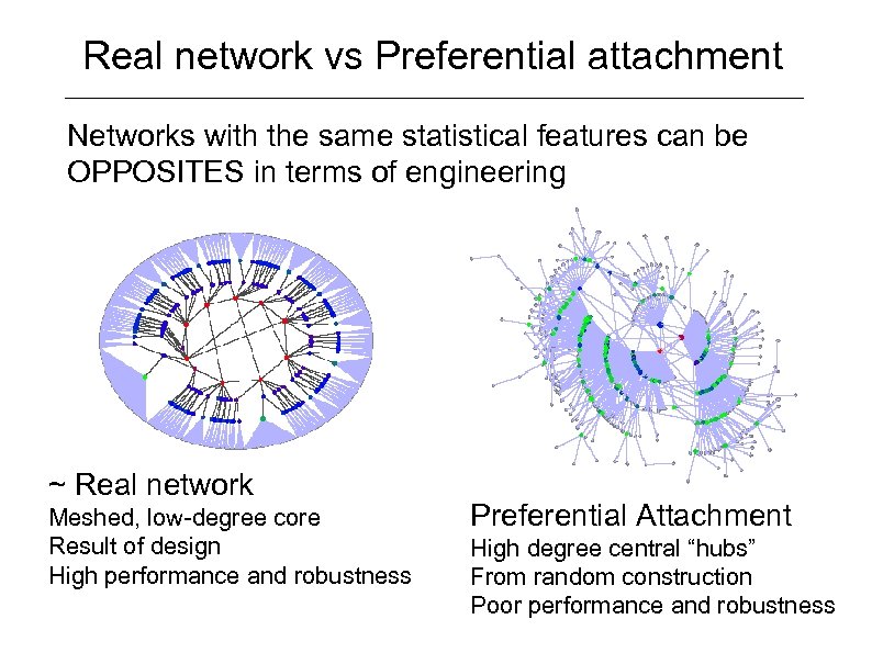Real network vs Preferential attachment Networks with the same statistical features can be OPPOSITES in terms of engineering ~ Real network Meshed, low-degree core Result of design High performance and robustness Preferential Attachment High degree central “hubs” From random construction Poor performance and robustness

Problems and Controversy § Scale-free claims: based critically on the implied relationship between power laws and a network structure that has highly connected “central hubs” § The scale-free models ignore all system-specific details in making their claims § Not all networks with power law degree distributions have properties of scale free networks (The Internet is just one example!) Building a model to replicate power law data is no more than curve fitting (descriptive, not explanatory) Ignore architecture e. g. hardware, protocol stack Ignore objectives e. g. performance Ignore constraints e. g. geography, economics Conclusion The scale-free claims of the Internet are not merely wrong, they suggest properties that are opposite to the real thing Fundamental difference: random vs. designed

Outline 1. Organization of the Internet 2. Evolution of the Internet 3. Internet Topology modelling Network properties Random Graphs models and generators Structural models and generators Topology measurements Power Law relationships Degree-based models and generators Internet topology metrics

Internet Topology Metrics A network topology is characterized by topological parameters, or topology metrics like: Average degree Distribution (DD) Joint Degree Distribution (JDD) a. k. a Degree correlation Clustering Rich club coefficient (RCC) Distance Betweenness Spectrum

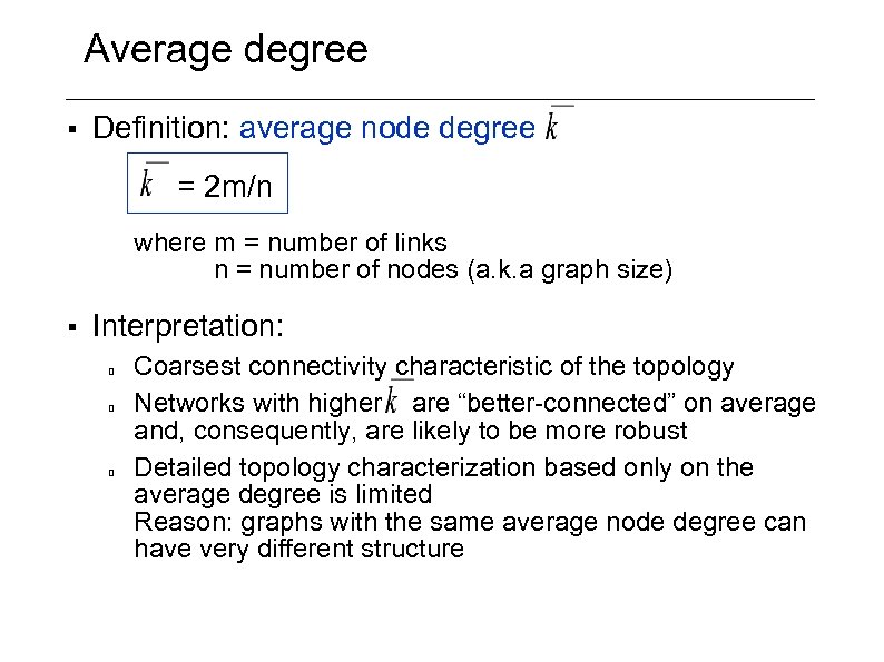Average degree § Definition: average node degree = 2 m/n where m = number of links n = number of nodes (a. k. a graph size) § Interpretation: Coarsest connectivity characteristic of the topology Networks with higher are “better-connected” on average and, consequently, are likely to be more robust Detailed topology characterization based only on the average degree is limited Reason: graphs with the same average node degree can have very different structure

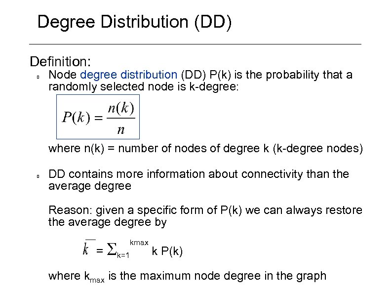Degree Distribution (DD) Definition: Node degree distribution (DD) P(k) is the probability that a randomly selected node is k-degree: where n(k) = number of nodes of degree k (k-degree nodes) DD contains more information about connectivity than the average degree Reason: given a specific form of P(k) we can always restore the average degree by = k=1 kmax k P(k) where kmax is the maximum node degree in the graph

Degree Distribution § Interpretation Most frequently used topology characteristic [Faloutsos 99] observation that Internet’s degree distribution (both router and AS-level) follows a power law had significant impact on network topology research – – Smooth power law degree distribution indicates – § Structural Internet models before failed to exhibit power laws organized hierarchy existence among ASes [Tangmunarunkit 02]: topologies derived from structural generators that incorporated hierarchies of AS tiers did not have much in common with topologies obtained from real observed data Indicates no organized tiers among ASes. The power law distribution also implies substantial variability associated with degrees of individual nodes Note: Node DD tells how many nodes of a given degree are in the network but it does NOT provide information on the interconnection between these nodes Reason: given P(k), structure of the neighborhood of the average node of a given degree is still unknown

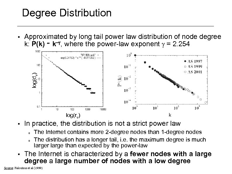Degree Distribution Approximated by long tail power law distribution of node degree k: P(k) ∼ k-g, where the power-law exponent g = 2. 254 log(dv) § log(rv) § In practice, the distribution is not a strict power law § The Internet contains more 2 -degree nodes than 1 -degree nodes The distribution has a longer tail, i. e. the maximum degree is much larger large than expected by the power-law The Internet is characterized by a fewer nodes with a large degree a large number of nodes with a low degree Source: Faloutsos et al (1999)

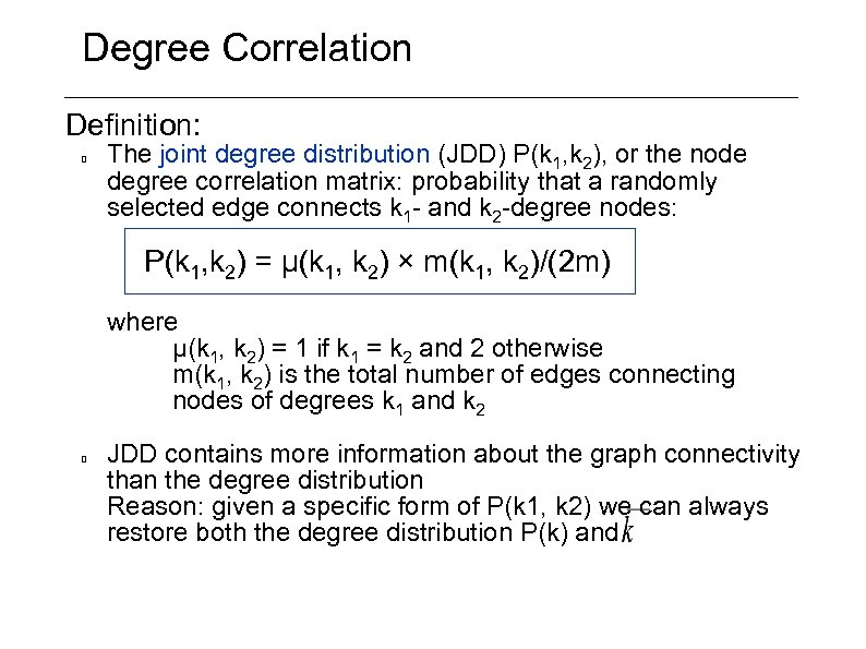Degree Correlation Definition: The joint degree distribution (JDD) P(k 1, k 2), or the node degree correlation matrix: probability that a randomly selected edge connects k 1 - and k 2 -degree nodes: P(k 1, k 2) = μ(k 1, k 2) × m(k 1, k 2)/(2 m) where μ(k 1, k 2) = 1 if k 1 = k 2 and 2 otherwise m(k 1, k 2) is the total number of edges connecting nodes of degrees k 1 and k 2 JDD contains more information about the graph connectivity than the degree distribution Reason: given a specific form of P(k 1, k 2) we can always restore both the degree distribution P(k) and

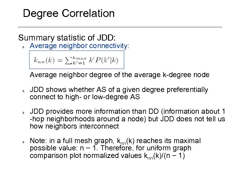Degree Correlation Summary statistic of JDD: Average neighbor connectivity: Average neighbor degree of the average k-degree node JDD shows whether AS of a given degree preferentially connect to high- or low-degree AS JDD provides more information than DD (information about 1 -hop neighborhoods around a node) but JDD does not tell us how neighbors interconnect Note: in a full mesh graph, knn(k) reaches its maximal possible value: n − 1. Therefore, for uniform graph comparison plot normalized values knn(k)/(n − 1)

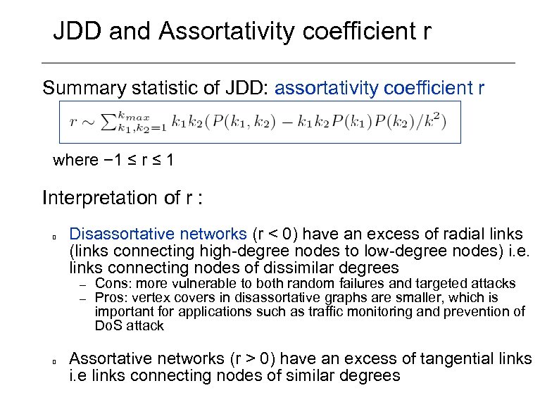JDD and Assortativity coefficient r Summary statistic of JDD: assortativity coefficient r where − 1 ≤ r ≤ 1 Interpretation of r : Disassortative networks (r < 0) have an excess of radial links (links connecting high-degree nodes to low-degree nodes) i. e. links connecting nodes of dissimilar degrees – – Cons: more vulnerable to both random failures and targeted attacks Pros: vertex covers in disassortative graphs are smaller, which is important for applications such as traffic monitoring and prevention of Do. S attack Assortative networks (r > 0) have an excess of tangential links i. e links connecting nodes of similar degrees

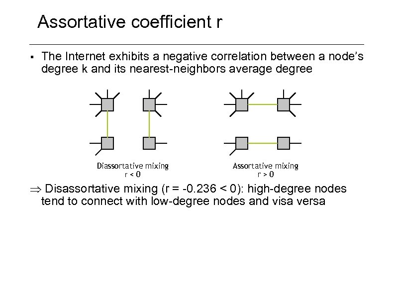Assortative coefficient r § The Internet exhibits a negative correlation between a node’s degree k and its nearest-neighbors average degree Diassortative mixing r<0 Assortative mixing r>0 Disassortative mixing (r = -0. 236 < 0): high-degree nodes tend to connect with low-degree nodes and visa versa

Likelihood S § [Li 04] introduces likelihood S (structural metric) Definition: sum of products of degrees of adjacent nodes S(g) = Si, j ki kj S measures randomness to differentiate between multiple graphs with the same DD (measures how “hub-like” the network core is) – (ki = degree of node i) (where node i, j are connected) S depends on graph structure, not the generation mechanism S is linearly related to the assortativity coefficient S is used as measure of graph randomness: a topology with low likelihood is not random; it results from some sophisticated evolution processes involving specific design purposes – – S provides a measure of the amount of order, e. g. , engineering design constraints, present in a given topology Router-level topologies are not “very random” but instead the result of sophisticated engineering design

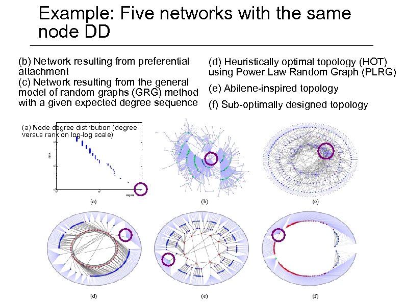Example: Five networks with the same node DD (b) Network resulting from preferential attachment (c) Network resulting from the general model of random graphs (GRG) method with a given expected degree sequence (a) Node degree distribution (degree versus rank on log-log scale) (d) Heuristically optimal topology (HOT) using Power Law Random Graph (PLRG) (e) Abilene-inspired topology (f) Sub-optimally designed topology

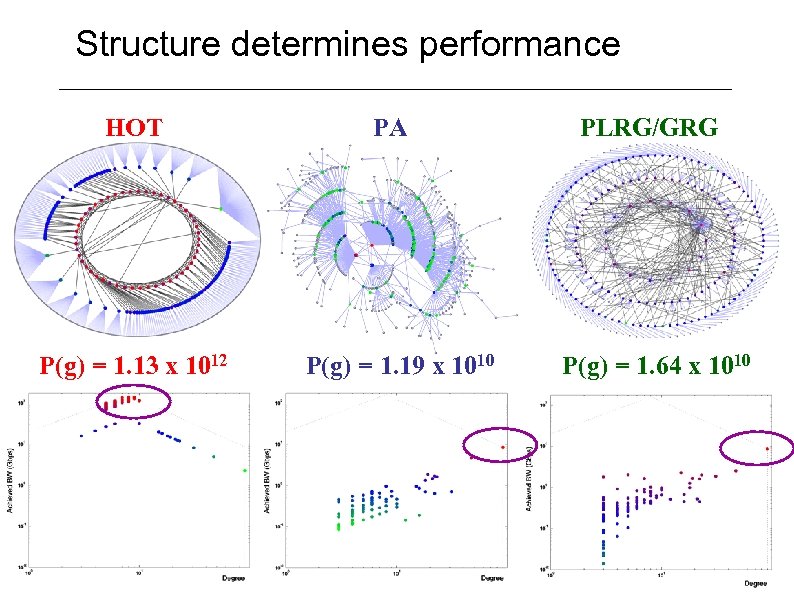Structure determines performance HOT P(g) = 1. 13 x 1012 PA P(g) = 1. 19 x 1010 PLRG/GRG P(g) = 1. 64 x 1010

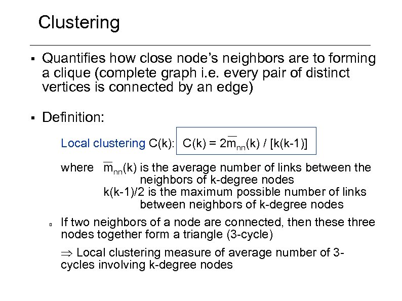Clustering § Quantifies how close node’s neighbors are to forming a clique (complete graph i. e. every pair of distinct vertices is connected by an edge) § Definition: Local clustering C(k): C(k) = 2 mnn(k) / [k(k-1)] where mnn(k) is the average number of links between the neighbors of k-degree nodes k(k-1)/2 is the maximum possible number of links between neighbors of k-degree nodes If two neighbors of a node are connected, then these three nodes together form a triangle (3 -cycle) Local clustering measure of average number of 3 cycles involving k-degree nodes

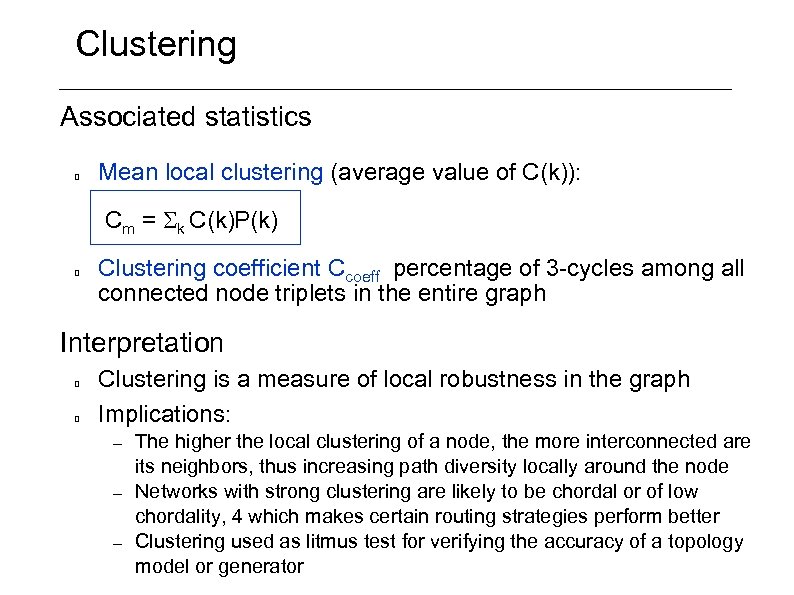Clustering Associated statistics Mean local clustering (average value of C(k)): Cm = k C(k)P(k) Clustering coefficient Ccoeff percentage of 3 -cycles among all connected node triplets in the entire graph Interpretation Clustering is a measure of local robustness in the graph Implications: – – – The higher the local clustering of a node, the more interconnected are its neighbors, thus increasing path diversity locally around the node Networks with strong clustering are likely to be chordal or of low chordality, 4 which makes certain routing strategies perform better Clustering used as litmus test for verifying the accuracy of a topology model or generator

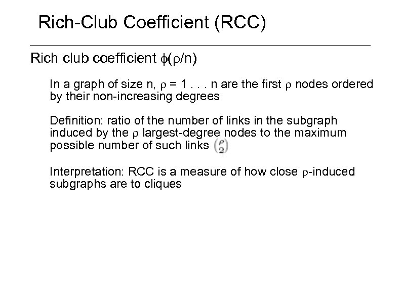Rich-Club Coefficient (RCC) Rich club coefficient f(r/n) In a graph of size n, r = 1. . . n are the first r nodes ordered by their non-increasing degrees Definition: ratio of the number of links in the subgraph induced by the r largest-degree nodes to the maximum possible number of such links Interpretation: RCC is a measure of how close r-induced subgraphs are to cliques

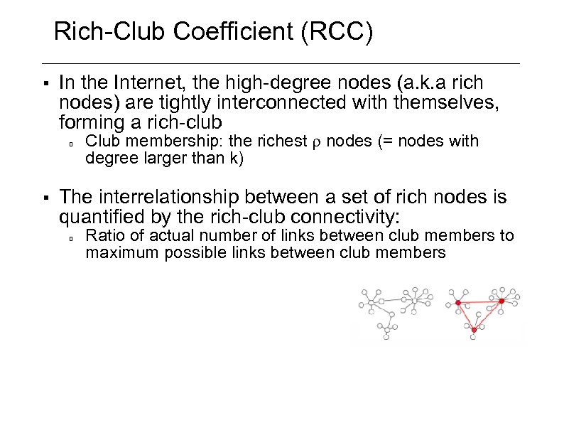Rich-Club Coefficient (RCC) § In the Internet, the high-degree nodes (a. k. a rich nodes) are tightly interconnected with themselves, forming a rich-club § Club membership: the richest r nodes (= nodes with degree larger than k) The interrelationship between a set of rich nodes is quantified by the rich-club connectivity: Ratio of actual number of links between club members to maximum possible links between club members

Distance § Definition: § The distance distribution d(x) is the number of pairs of nodes at a distance x, divided by the total number of pairs n 2 (self-pairs included) Associated statistics with distance distribution of a graph Average distance dm Standard deviation s (a. k. a distance distribution width since distance distributions in Internet graphs have a characteristic Gaussian-like shape)

Distance Interpretation Distance distribution is important for routing: – – Distance distribution plays a vital role in robustness of the network to worms – – Distance-based locality-sensitive approach root of most modern routing algorithms: performance of routing algorithms depend mostly on the distance distribution Short average distance and narrow distance distribution width break the efficiency of traditional hierarchical routing: root causes of interdomain routing scalability issues in the Internet Worms can quickly contaminate a network that has small distances between nodes Topology models (that accurately reproduce observed distance distributions) will benefit development of techniques to quarantine the network from worms Expansion metric: renormalized version of distance distribution d(x) – Critical metric for topology comparison analysis

Betweeness § Betweenness § Measures the number of shortest paths traversing a vertex(node) or edge(link) if each individuals send a message to all other individuals Estimation of the potential traffic load (flow of information) on this node/link assuming uniformly distributed traffic following shortest paths Definition sij : number of shortest paths between nodes i and j y : either a node or link sij(y) : number of shortest paths between i and j going through y Betweeness By = ij sij(y)/sij The maximum possible value for node and link betweenness is n(n − 1) to compare betweenness in graphs of different sizes, normalization by n(n − 1)

Betweeness Interpretation Important metric for traffic engineering applications that try to estimate potential traffic load on nodes/links and potential congestion points in a given topology Critical for evaluating the accuracy of topology sampling by tree-like probes (e. g. skitter and BGP) – – The broader the betweenness distribution, the higher the statistical accuracy of the sampled graph Note: exploration process statistically focuses on nodes/links with high betweenness thus providing an accurate sampling of the distribution tail and capturing relevant statistical information Note: link betweenness is not a measure of centrality but a measure of a certain combination of link centrality and radiality

Spectrum § Definition A : n × n adjacency matrix of a graph constructed by setting the value of its element as – – § aij = aji = 1 if there is a link between nodes i and j all other elements have value 0 Scalar are the eigenvalue and vector v the eigenvector of A if A v = v Spectrum of a graph is the set of eigenvalues of its adjacency matrix A Interpretation: (one of the) most important global characteristics of the topology Provides bounds for critical graph characteristics such as distance-related parameters, expansion properties, and values related to separator problems estimating graph resilience under node/link removal Most networks with high values as eigenvalues have small diameter, expand faster, and are more robust

Spectrum § Example of spectrum-related metrics Robustness of network – – – Performance: Max. traffic throughput of network – § Relation to spectrum: network conductance can be tightly estimated by the gap between the first and second largest eigenvalues Application to Traffic engineering § Critical metric for topology comparison analysis Measure of network robustness under link removal (equals minimum balanced cut size of a graph) Relation to spectrum: graph’s largest eigenvalues provide bounds on network robustness with respect to both link and node removals Graphs with larger eigenvalues have, in general, more node - and link-disjoint paths to choose from Spectral analysis Powerful tool for detailed investigation of network structure Example: discovering clusters of highly interconnected nodes and revealing AS hierarchy

Scaling dependency on Topology Internet topological properties characterized by Node degree distribution: approximated by long tail power law distribution P(k) ∼ k-γ, γ = 2. 254 (scaling index) The Internet is characterized by a fewer nodes with a large degree a large number of nodes with a low degree Node degree correlation: negative correlation between a node’s degree k and its nearest-neighbors average degree Disassortative mixing (r = -0. 236 < 0): high-degree nodes tend to connect with low-degree nodes and visa versa Clustering: large numbers of short subgraphs (3 -/4 -cycles) >< regular tree structures basic units for routing redundancy and community clustering Shortest Path Length: The average length of shortest paths between all pairs of nodes on the Internet is just over 3 hops Average AS-path length ~constant (avg. 3, 4) >< hierarchical routing (performs well for graphs with large distances between nodes)

Backup Material

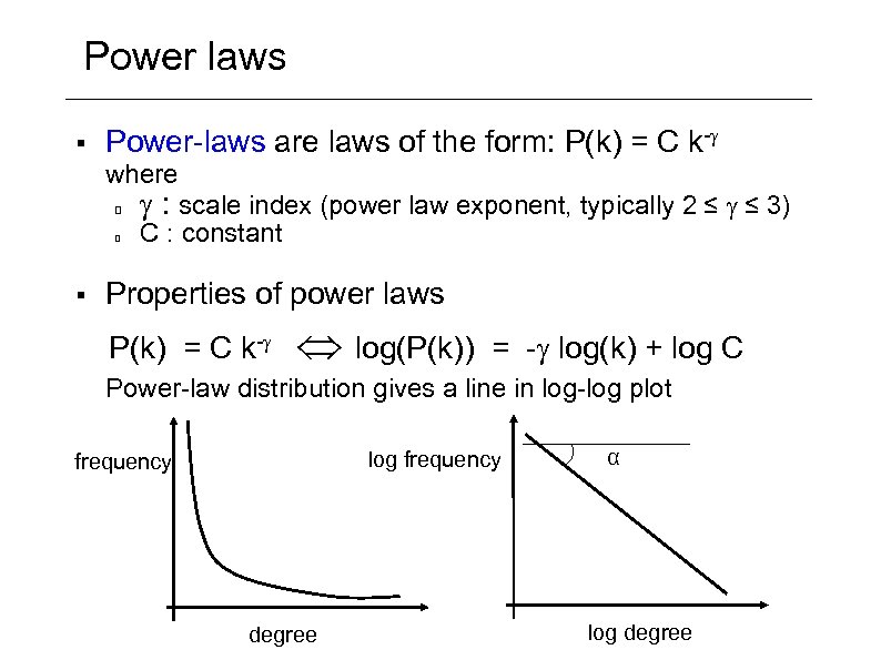Power laws § Power-laws are laws of the form: P(k) = C k-g where § g : scale index (power law exponent, typically 2 ≤ g ≤ 3) C : constant Properties of power laws P(k) = C k-g log(P(k)) = -g log(k) + log C Power-law distribution gives a line in log-log plot log frequency degree α log degree

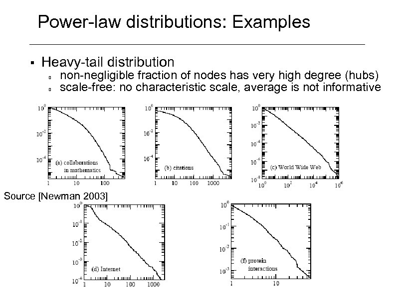Power-law distributions: Examples § Heavy-tail distribution non-negligible fraction of nodes has very high degree (hubs) scale-free: no characteristic scale, average is not informative Source [Newman 2003]

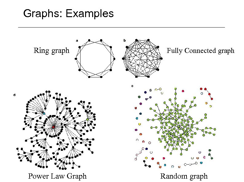Graphs: Examples Ring graph Power Law Graph Fully Connected graph Random graph

References

References [Aiello 00] W. Aiello, F. Chung, and L. Lu. A Random Graph Model for Massive Graphs. In Proceedings of ACM Symposium on Theory of Computing, pp. 171— 180, 2000. [Aiello 01] W. Aiello, F. Chung, and L. Lu. A Random Graph Model for Power Law Graphs. Experimental Math. 10, pp. 53— 66, 2001. [Aiello 02] W. Aiello, F. Chung, and L. Lu. Random Evolution in Massive. Graphs. In Handbook on Massive Data Sets, vol. 2, pp. 97– 122, Spinger, 2002. [Albert 00 a] Reka Albert, Hawoong Jeong, and Albert-Laszlo Barabasi, Attack and error tolerance of complex networks, Nature 406, pp. 378 -382, 2000. [Albert 00 b] R. Albert and A. L. Barabasi, Topology of Evolving Networks: Local Events and Universality, Physical Review Letters, 85(24): 5234 -5237, 2000. [Albert 02] R. Albert and A. -L. Barabási, Statistical mechanics of complex networks, Reviews of Modern Physics, vol. 74, pp. 47 -97, 2002. [Alderson 05 a] D. Alderson, L. Li, W. Willinger, J. C. Doyle, Understanding Internet Topology: Principles, Models, and Validation. ACM/IEEE Trans. on Networking 13(6), 2005. [Alderson 05 b] D. Alderson and W. Willinger, A contrasting look at self-organization in the Internet and nextgeneration communication networks. IEEE Comm. Magazine. July 2005. [Barabasi 99 a] Albert-Laszlo Barabasi and Reka Albert, Emergence of scaling in random networks, Science, vol. 286(5439), pp. 509 -512, 1999. [Barabasi 99 b] A. -L. Barabasi, R. Albert, and H. Jeong, Mean-field theory for scale-free random networks, Physica A 272, pp. 173 -187, 1999. [Barabasi 01] A. -L. Barabasi, E. Ravasz, and T. Vicsek. Deterministic scale- free networks, Physica A, 299: 599, 2001. [Barabasi 03 a] Albert-Laszlo Barabasi, Linked: How Everything Is Connected to Everything Else and What It Means (Plume, 2003). [Barabasi 03 b] A. -L. Barabasi, Z. Dezso, E. Ravasz, S. H. Yook, and Z. Oltvai. Scale-free and Hierarchical Structures in Complex Networks, AIP Conference Proceedings, 2003. [Bollobas 01] B. Bollobas, O. Riordan, J. Spencer, and G. Tusnady. The Degree Sequence of a Scale. Free Random Process. Random Structures and Algorithms, 18(3): 279— 290, 2001. [Bollobas 03 a] Bela Bollobas and Oliver Riordan, Robustness and Vulnerability of Scale-Free Random Graphs, Internet Mathematics, vol. 1, no. 1, pp. 1 -35, 2003. [Bollobas 03 b] Bela Bollobas and Oliver Riordan, Coupling Scale-Free and Classical Random Graphs, Internet Mathematics, vol. 1, no. 2, pp. 215 -225, 2003.

References [Bollobas 04] B. Bollobas and O. Riordan. The Diameter of a Scale-Free Random Graph, Combinatorica, vol. 24, no. 1, pp. 5– 34, 2004. [Bu 02] T. Bu and D. Towsley, "On distinguishing between Internet power law topology generators, " in Proc. of IEEE INFOCOM, Dec. 2002. [Carlson 99]J. M. Carlson and J. Doyle, "Highly optimized tolerance: A mechanism for power laws in designed systems, " Physical Review E, vol. 60, pp. 1412 -1427, 1999. [Chang 03] H. Chang, S. Jamin, and W. Willinger, Internet connectivity at the AS-level: An optimization- driven modeling approach, in Mo. Me. Tools, 2003. [Chang 04] H. Chang, R. Govindan, S. Jamin, S. J. Shenker, and W. Willinger, Towards capturing representative AS-level Internet topologies, Computer Networks Journal, vol. 44, pp. 737 -755, April 2004. [Chang 06] H. Chang, S. Jamin, and W. Willinger, To peer or not to peer: Modeling the evolution of the Internet's AS-level topology, in Proc. IEEE INFOCOM, 2006. [Chen 02] Q. Chen, H. Chang, R. Govindan, S. Jamin, S. J. Shenker, and W. Willinger, The origin of power laws in Internet topologies revisited, in Proc. IEEE INFOCOM, June 2002. [Chung 03 a] F. Chung and L. Lu. The Average Distance in a Random Graph with Given Expected Degrees. Internet Mathematics, vol. 1, no. 1, pp. 91– 114, 2003. [Chung 03 b] Fan Chung, Linyuan Lu, and Van Vu. The Spectra of Random Graphs with Given Expected Degrees. Internet Mathematics, vol. 1, no. 3, pp. 257 -275, 2003. [Chung 04] Fan Chung and Linyuan Lu. Coupling Online and Offline Analyses for Random Power Law Graphs. Internet Mathematics, vol. 1, no. 4, pp. 409 -461, 2004. [Cooper 04] Colin Cooper, Alan Frieze, and Juan Vera. Random Deletion in a Scale-Free Random Graph Process. Internet Mathematics, vol. 1, no. 4, pp. 463 -483, 2004. [Dall. Asta 05] L. Dall'Asta, I. Alvarez-Hamelin, A. Barrat, A. Vazquez, and A. Vespignani, "Exploring networks with traceroute-like probes: Theory and simulations, " Theoretical Computer Science, Special Issue on Complex Networks, 2005. [Dimitropoulos 06] X. Dimitropoulos, D. Krioukov, G. Riley, and K. Claffy, Revealing the Autonomous System taxonomy: The machine learning approach, in Proc. PAM, March 2006. [Dimitropoulos 07] X. Dimitropoulos, D. Krioukov, M. Fomenkov, B. Huffaker, Y. Hyun, K. Claffy, and G. Riley, AS relationships: Inference and validation, Computer Communication Review, vol. 37, no. 1, 2007 [Dorogovstev 03] S. N. Dorogovtsev and J. F. F. Mendes, Evolution of Networks. Oxford, England: Oxford University Press, 2003.

References [Doyle 05] J. C. Doyle, D. Alderson, L. Li, S. Low, M. Roughan, S. Shalunov, R. Tanaka, and W. Willinger, The "robust yet fragile" nature of the Internet. PNAS 102(41), 2005. [Erdos 60 a] P. Erdos, and A. Rényi. On the evolution of random graphs. Publ. Math. Inst. Hung. Acad. Sci. 5, pp. 17 -60, 1960. [Erdos 60 b] P. Erdos and T. Gallai. Graphs with prescribed degrees of vertices. Mat. Lapok (Hungarian), 11, pp. 264 -274, 1960. [Erdos 59] P. Erdos and A. Renyi. On random graphs I Publ. Math. (Debrecen) 9, pp. 290 -297, 1959. [Fabrikant 02] A. Fabrikant, E. Koutsoupias, and C. H. Papadimitriou. “Heuristically Optimized Tradeoffs: A New Paradigm for Power Laws in the Internet. In Proceedings of ICALP, Lecture Notes in Computer Science 2380, pp. 110— 122, Springer—Verlag, 2002. [Faloutsos 99] M. Faloutsos, P. Faloutsos, and C. Faloutsos, On power-law relationships of the Internet topology, in Proc. ACM SIGCOMM 1999 and in ACM Computer Communication Review, 29, pp. 251263, 1999. [Jin 00] C. Jin, Q. Chen, and S. Jamin, "INET topology generator", Technical Report, EECS Department, University of Michigan, 2000. [Jin 02] S. Jin and A. Bestavros, "Small-world internet topologies: Possible causes and implications on scalability of end-system multicast", Technical Report, Boston University, 2002. [Krapivsky 01] P. L. Krapivsky and S. Redner, "Organization of growing random networks, " Physical Review E, vol. 63, no. 6, May 2001. [Krioukov 04] D. Krioukov, K. Fall, and X. Yang. Compact routing on Internet-like graphs. in Proc. IEEE INFOCOM, 2004. [Li 04] L. Li, D. Alderson, W. Willinger, and J. Doyle, A first-principles approach to understanding the Internet’s router-level topology, in Proc. ACM SIGCOMM, 2004. [Li 05] L. Li, D. Alderson, J. C. Doyle, and W. Willinger. Toward a Theory of Scale-Free Networks: Definition, Properties, and Implications. Internet Mathematics, vol. 2, no. 4, pp. 431 -523, 2005. [Mahadevan 06 a] P. Mahadevan, D. Krioukov, M. Fomenkov, B. Huffaker, X. Dimitropoulos, kc claffy, and A. Vahdat. The Internet AS-level topology: Three data sources and one definitive metric. Computer Communication Review, vol. 36, no. 1, 2006. [Mahadevan 06 b] P. Mahadevan, D. Krioukov, K. Fall, and A. Vahdat, Systematic topology analysis and generation using degree correlations, in Proc. ACM SIGCOMM, 2006. [Medina 00] A. Medina, I. Matta, and J. Byers, "On the origin of power laws in Internet topologies", ACM Computer Communication Review, vol. 30, no. 2, pp. 18 -28, April 2000. [Mihail 02] M. Mihail, C. H. Papadimitriou: On the Eigenvalue Power Law. RANDOM, pp. 254 -262, 2002.

References [Newman 02] M. E. J. Newman, Assortative Mixing in Networks, Phys. Rev. Lett. 89, 208701 (2002). [Newman 03] M. E. J. Newman, The Structure and Function of Complex Networks, SIAM Reviews, vol. 45, no. 2, pp. 167 -256, 2003. [Newman 05] M. E. J. Newman. Power laws, Pareto distributions and Zipfs law, Contemporary Physics, vol. 46, no. 5, pp. 323– 351, January 2005. [Oliveira 05]R. Oliveira and J. Spencer, Connectivity Transitions in Networks with Super-Linear Preferential Attachment, Internet Mathematics, vol. 2, no. 2, pp. 121 -163, 2002. [Palmer 01] C. Palmer, G. Siganos, M. Faloutsos, C. Faloutsos and P. Gibbons, The connectivity and faulttolerance of the Internet topology (NRDM 2001), Santa Barbara, CA, May 2001. [Radoslavov 00] P. Radoslavov, H. Tangmunarunkit, H. Yu, R. Govindan, S. Shenker, D. Estrin, On characterizing network topologies and analyzing their impact on protocol design, USC-CS- TR-00731, March 2000. [Serrano 06] M. A. Serrano, M. Boguna, and A. Daz-Guilera, Modeling the Internet, The European Physical Journal B, vol. 50, pp. 249 -254, 2006. [Siganos 03] G. Siganos, M. Faloutsos, P. Faloutsos, and C. Faloutsos, Power Laws and the AS-level Internet topology, Transactions on Networking, vol. 11, no. 4, pp. 514 -524, August 2003. [Tangmunarunkit 02] H. Tangmunarunkit, R. Govindan, S. Jamin, S. Shenker, W. Willinger, Network Topology Generators: Degree-Based vs. Structural, in Proc. of ACM SIGCOMM 2002. [Vukadinovic 02] D. Vukadinovic, P. Huang, T. Erlebach. On the Spectrum and Structure of Internet Topology Graphs. in Proc. I 2 CS 2002. [Waxman 98] Waxman, Routing of multipoint connections, IEEE JSAC, 1988. [Willinger 04 a] W. Willinger, D Alderson, J. C. Doyle, and L. Li, More "normal" than Normal: scaling distributions in complex systems. Proc. Winter Simulation Conference 2004. [Willinger 04 b] W. Willinger, D Alderson, and L. Li, A pragmatic approach to dealing with high-variability in network measurements, in Proc. ACM SIGCOMM, IMC 2004. [Xang 06] X. Wang and D. Loguinov, "Wealth-based evolution model for the Internet AS-level topology, " in Proc. IEEE INFOCOM, 2006. [Yook 02] S. -H. Yook, H. Jeong, and A. -L. Barabasi. Modeling the Internets large-scale topology, PNAS 99, 13382 -86 (2002). [Zegura 97] E. W. Zegura, K. L. Calvert and M. J. Donahoo. A Quantitative Comparison of Graph-based Models for Internet Topology. IEEE/ACM Transactions on Networking, vol. 5, no. 6, Dec. 1997. [Zhou 04] S. Zhou and R. J. Mondragon, Accurately modeling the Internet topology, Physical Review E, vol. 70, p. 066108, 2004.