EC 202 Worked Example 3 13 Frank Cowell

EC 202: Worked Example #3. 13 Frank Cowell April 2005 • This presentation covers exactly the material set out in the file Worked. Examples. pdf, but with the addition of a few graphics and comments • To start the presentation select SlideshowView Show or click on icon below left. • Mouse click or [Enter] to advance through slide show

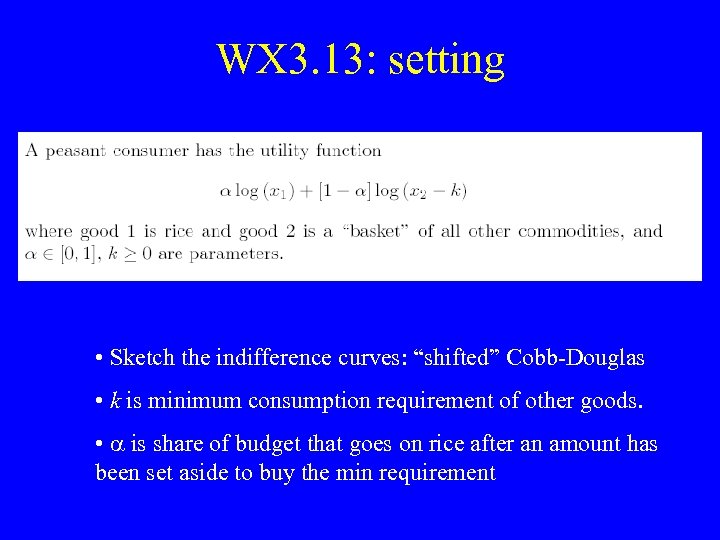WX 3. 13: setting • Sketch the indifference curves: “shifted” Cobb-Douglas • k is minimum consumption requirement of other goods. • a is share of budget that goes on rice after an amount has been set aside to buy the min requirement

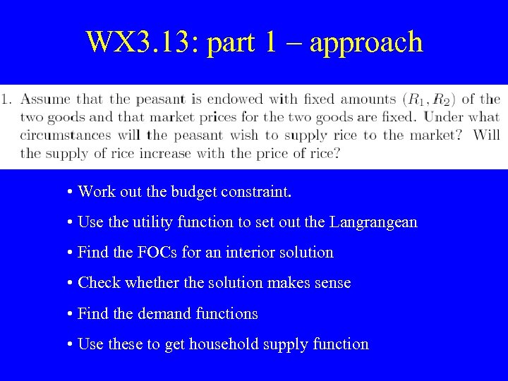WX 3. 13: part 1 – approach • Work out the budget constraint. • Use the utility function to set out the Langrangean • Find the FOCs for an interior solution • Check whether the solution makes sense • Find the demand functions • Use these to get household supply function

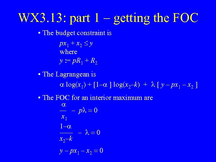WX 3. 13: part 1 – getting the FOC • The budget constraint is px 1 + x 2 y where y : = p. R 1 + R 2 • The Lagrangean is a log(x 1) + [1–a ] log(x 2–k) + l [ y – px 1 – x 2 ] • The FOC for an interior maximum are a — – pl = 0 x 1 1–a —— – l = 0 x 2–k y – px 1 – x 2 = 0

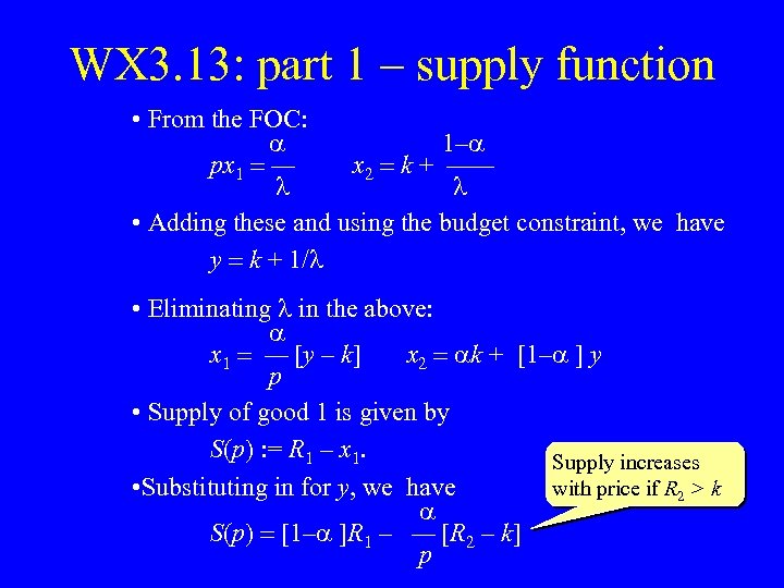WX 3. 13: part 1 – supply function • From the FOC: a 1–a px 1 = — x 2 = k + —— l l • Adding these and using the budget constraint, we have y = k + 1/l • Eliminating l in the above: a x 1 = — [y – k] x 2 = ak + [1–a ] y p • Supply of good 1 is given by S(p) : = R 1 – x 1. Supply increases • Substituting in for y, we have with price if R 2 > k a S(p) = [1–a ]R 1 – — [R 2 – k] p

WX 3. 13: part 2 • If ak + [1–a ] y c nothing changes from previous case. • Otherwise px 1 + c = y so that R 2 – c x 1 = R 1 + ——— p

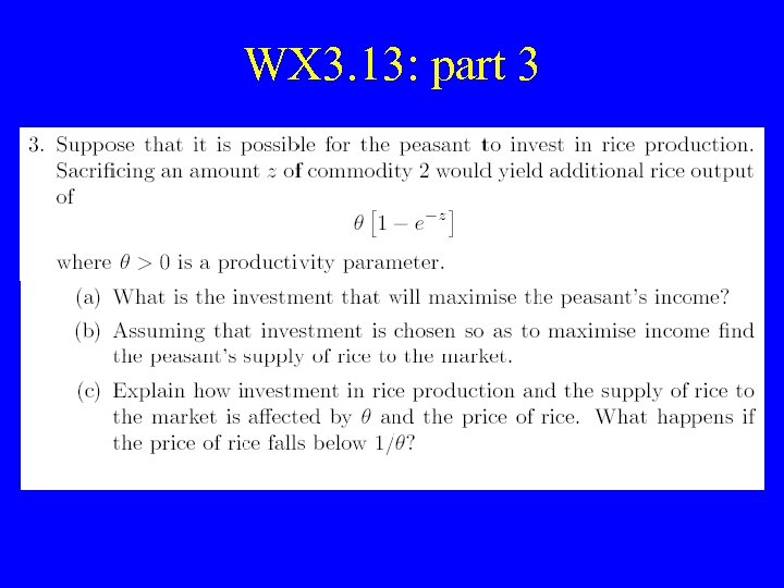WX 3. 13: part 3

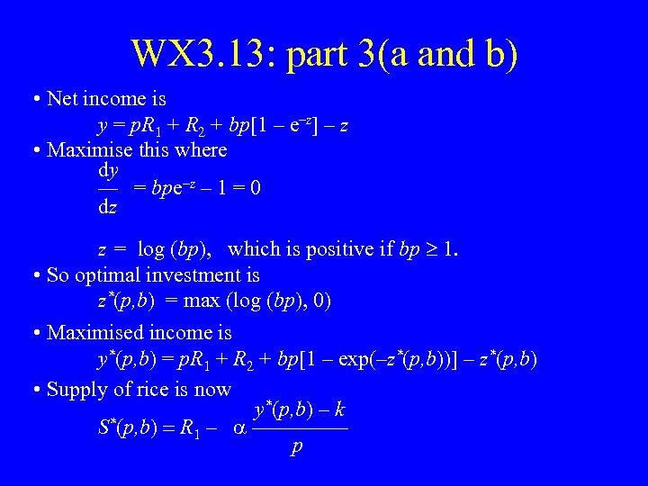WX 3. 13: part 3(a and b) • Net income is y = p. R 1 + R 2 + bp[1 – e–z] – z • Maximise this where dy — = bpe–z – 1 = 0 dz z = log (bp), which is positive if bp 1. • So optimal investment is z*(p, b) = max (log (bp), 0) • Maximised income is y*(p, b) = p. R 1 + R 2 + bp[1 – exp(–z*(p, b))] – z*(p, b) • Supply of rice is now y*(p, b) – k S*(p, b) = R 1 – a ————— p

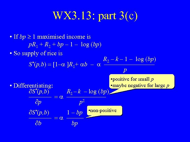WX 3. 13: part 3(c) • If bp 1 maximised income is p. R 1 + R 2 + bp – 1 – log (bp) • So supply of rice is R 2 – k – 1 – log (bp) S*(p, b) = [1–a ]R 1+ ab – a ————— p • Differentiating: S*(p, b) R 2 – k – log (bp) ———— = a ——————— p p 2 • positive for small p • maybe negative for large p S*(p, b) 1 – bp • non-positive ———— = a ——— b bp