Dynamic Efficiency & Hotelling’s Rule [adapted from S.

Dynamic Efficiency & Hotelling’s Rule [adapted from S. Hackett’s lecture notes]

Dynamic efficiency Recall static notion of Pareto efficient resource allocation is that one cannot change how resources are split to generate larger gains from trade (without making some one else worse off) In contrast, dynamic efficient resource allocation is that one cannot shift production from one time period to another and generate a larger present value of gains from trade summed across all time periods.

Dynamic efficiency The notion of dynamic efficiency is an intuitive concept. First, let’s consider the concept of present (discounted) value. Would you rather have $10, 000 in cash right now or 10 years from now? Why (or why not)?

Dynamic efficiency Reasons why most people would rather have $10, 000 today instead of 10 years from now: • If we anticipate inflation (rising prices over time), then the purchasing power of $10, 000 will shrink over time. • If we take the $10, 000 today and invest it in, say, government bonds, then we will have more than $10, 000 in 10 years.

Dynamic efficiency Reasons why most people would rather have $10, 000 today instead of 10 years from now (continued): • Pure rate of time preference: I want good things now and would rather wait for bad things. I don’t know if I will be alive in 10 years, so why wait? • Strong current needs (e. g. , college expenses, health care expenses, basic food and shelter needs) heightens one’s pure rate of time preference.

Dynamic efficiency Suppose that you have inherited $10, 000, which will be held in trust for you for 10 years. • What is the least amount of cash you would accept from me RIGHT NOW that would make you willing to sign over the inheritance to me? • Your answer to that question is your present (discounted) value of that future $10, 000 payment.

Dynamic efficiency As an aside, why might your present discounted value of a $10, 000 payment 10 years in the future differ from that of someone else? Different life circumstances, different investment opportunities. Other?

Dynamic efficiency Note: The discount rate (like an interest rate) reflects the time value of money : • The rate at which the present value of a payment shrinks as the time of payment is pushed off further into the future • The rate at which the future value of current interest-earning savings grows over time.

Dynamic efficiency Since different people have different discount rates, then at the prevailing market interest rate, some people are lenders (financial investors), while others are borrowers. As with market equilibrium price, the equilibrium market interest rate reflects a balancing of the discount rates of those supplying and demanding loanable funds.

Dynamic efficiency Finance is an application of economics that focuses on time value of money. We will limit ourselves to an elementary application of the time value of money.

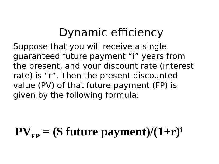
Dynamic efficiency Suppose that you will receive a single guaranteed future payment “i” years from the present, and your discount rate (interest rate) is “r”. Then the present discounted value (PV) of that future payment (FP) is given by the following formula: PV FP = ($ future payment)/(1+r) i

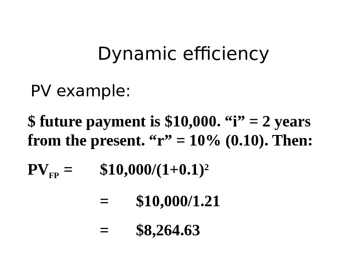
Dynamic efficiency PV example: $ future payment is $10, 000. “i” = 2 years from the present. “r” = 10% (0. 10). Then: PV FP = $10, 000/(1+0. 1) 2 = $10, 000/1. 21 = $8, 264.

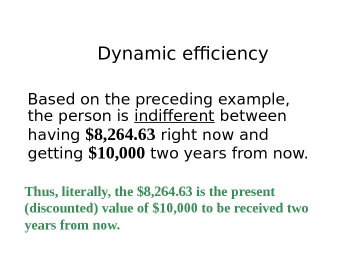
Dynamic efficiency Based on the preceding example, the person is indifferent between having $8, 264. 63 right now and getting $10, 000 two years from now. Thus, literally, the $8, 264. 63 is the present (discounted) value of $10, 000 to be received two years from now.

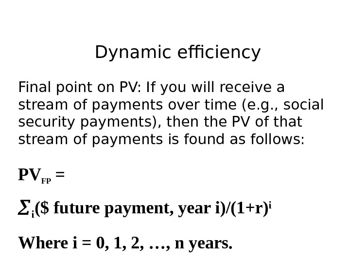
Dynamic efficiency Final point on PV: If you will receive a stream of payments over time (e. g. , social security payments), then the PV of that stream of payments is found as follows: PV FP = i ($ future payment, year i)/(1+r) i Where i = 0, 1, 2, …, n years.

Dynamic efficiency Moving on… Our analysis of dynamic efficiency will be based on a highly simplified modeling framework, which will provide an accessible introduction to the topic, as well as important insights, without overwhelming you with complex mathematics.

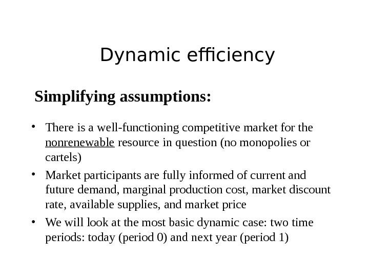
Dynamic efficiency Simplifying assumptions: • There is a well-functioning competitive market for the nonrenewable resource in question (no monopolies or cartels) • Market participants are fully informed of current and future demand, marginal production cost, market discount rate, available supplies, and market price • We will look at the most basic dynamic case: two time periods: today (period 0) and next year (period 1)

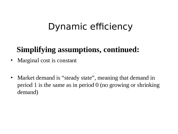
Dynamic efficiency Simplifying assumptions, continued: • Marginal cost is constant • Market demand is “steady state”, meaning that demand in period 1 is the same as in period 0 (no growing or shrinking demand)

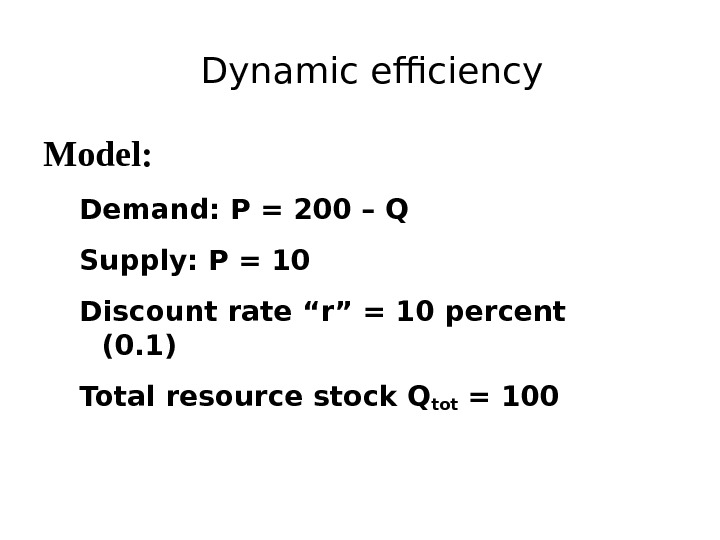
Dynamic efficiency Model: Demand: P = 200 – Q Supply: P = 10 Discount rate “r” = 10 percent (0. 1) Total resource stock Qtot =

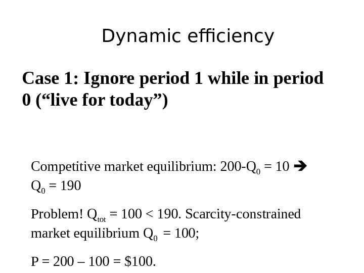
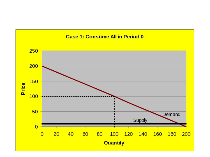
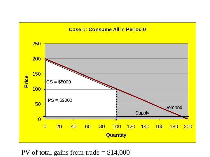
Dynamic efficiency Case 1: Ignore period 1 while in period 0 (“live for today”) Competitive market equilibrium: 200 -Q 0 = 10 Q 0 = 190 Problem! Q tot = 100 < 190. Scarcity-constrained market equilibrium Q 0 = 100; P = 200 – 100 = $100.

Case 1: Consume All in Period 0 050100150200250 0 20 40 60 80 100 120 140 160 180 200 Quantity. P rice Demand Supply

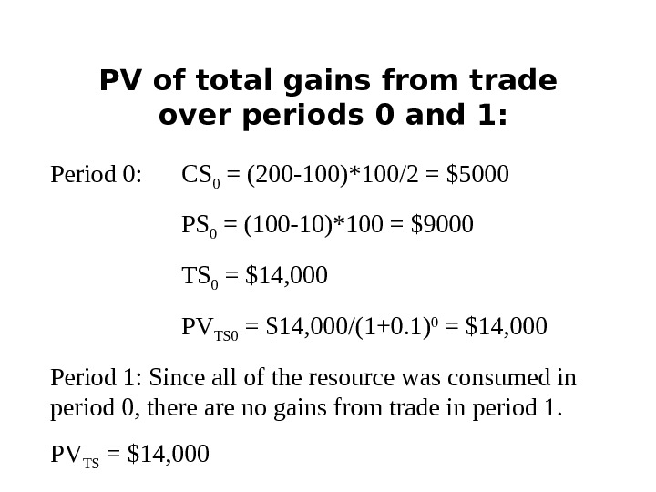
PV of total gains from trade over periods 0 and 1: Period 0: CS 0 = (200 -100)*100/2 = $5000 PS 0 = (100 -10)*100 = $9000 TS 0 = $14, 000 PV TS 0 = $14, 000/(1+0. 1) 0 = $14, 000 Period 1: Since all of the resource was consumed in period 0, there are no gains from trade in period 1. PV TS = $14,

Case 1: Consume All in Period 0 050100150200250 0 20 40 60 80 100 120 140 160 180 200 Quantity. P rice Demand Supply CS = $5000 PS = $9000 PV of total gains from trade = $14,

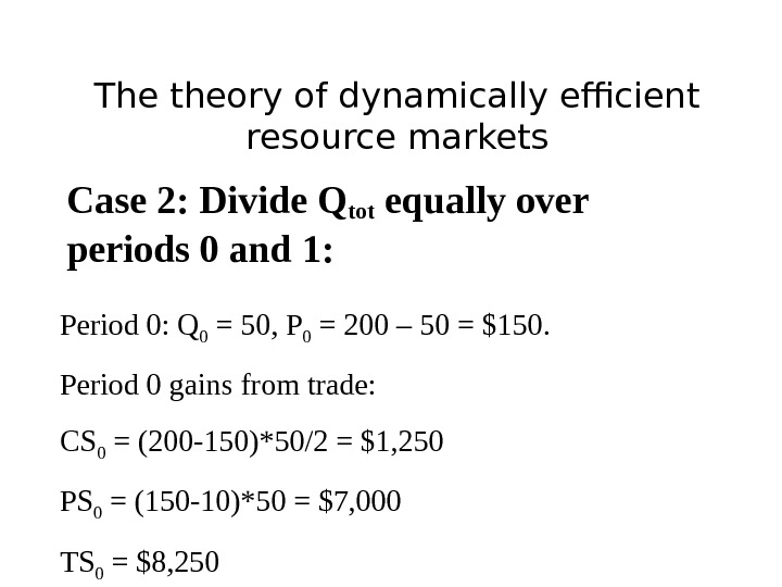
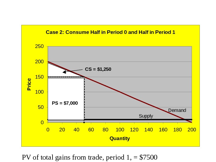
The theory of dynamically efficient resource markets Case 2: Divide Qtot equally over periods 0 and 1: Period 0: Q 0 = 50, P 0 = 200 – 50 = $150. Period 0 gains from trade: CS 0 = (200 -150)*50/2 = $1, 250 PS 0 = (150 -10)*50 = $7, 000 TS 0 = $8,

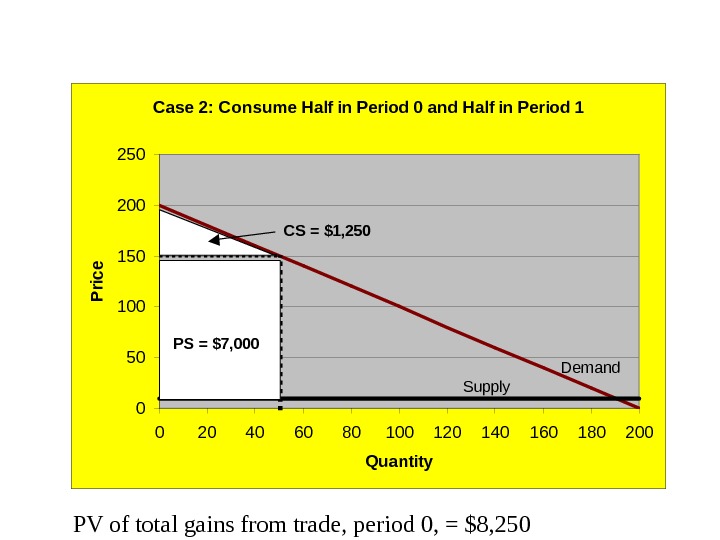
PV of total gains from trade, period 0, = $8, 250 Case 2: Consume Half in Period 0 and Half in Period 1 050100150200250 0 20 40 60 80 100 120 140 160 180 200 Quantity. P rice Demand Supply CS = $1, 250 PS = $7,

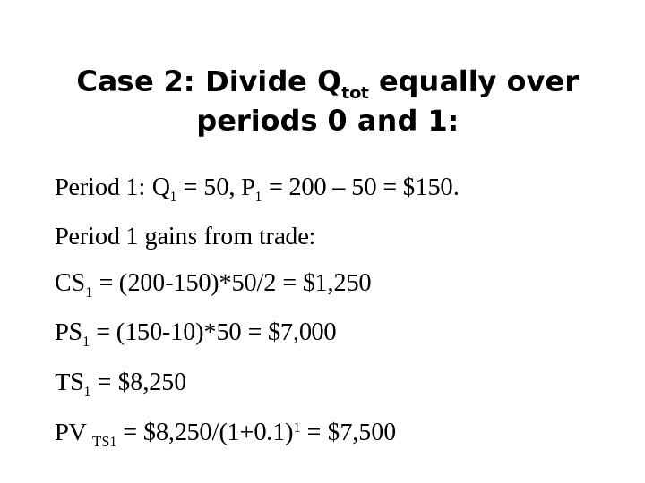
Case 2: Divide Q tot equally over periods 0 and 1: Period 1: Q 1 = 50, P 1 = 200 – 50 = $150. Period 1 gains from trade: CS 1 = (200 -150)*50/2 = $1, 250 PS 1 = (150 -10)*50 = $7, 000 TS 1 = $8, 250 PV TS 1 = $8, 250/(1+0. 1) 1 = $7,

PV of total gains from trade, period 1, = $7500 Case 2: Consume Half in Period 0 and Half in Period 1 050100150200250 0 20 40 60 80 100 120 140 160 180 200 Quantity. P rice Demand Supply CS = $1, 250 PS = $7,

Case 2: Divide Q tot equally over periods 0 and 1: Sum of the PV of total gains from trade over periods 0 and 1: $8, 250 + $7500 = $15, 750 Note that $15, 750 in PV of total gains from trade from dividing the resource equally over periods 0 and 1 EXCEEDS the $14, 000 in total gains from trade when we consumed all of the resource in period 0. Thus equal division is closer to being dynamically efficient.

Methods for solving for the dynamically efficient allocation of the fixed stock of resource over time: Hotelling’s rule : The dynamically efficient allocation occurs when the PV of marginal profit (also known as marginal scarcity rent or marginal Hotelling rent) for the last unit consumed is equal across the various time periods.

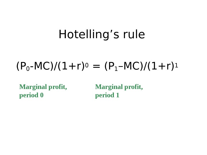
Hotelling’s rule (P 0 -MC)/(1+r) 0 = (P 1 –MC)/(1+r) 1 Marginal profit, period 0 Marginal profit, period

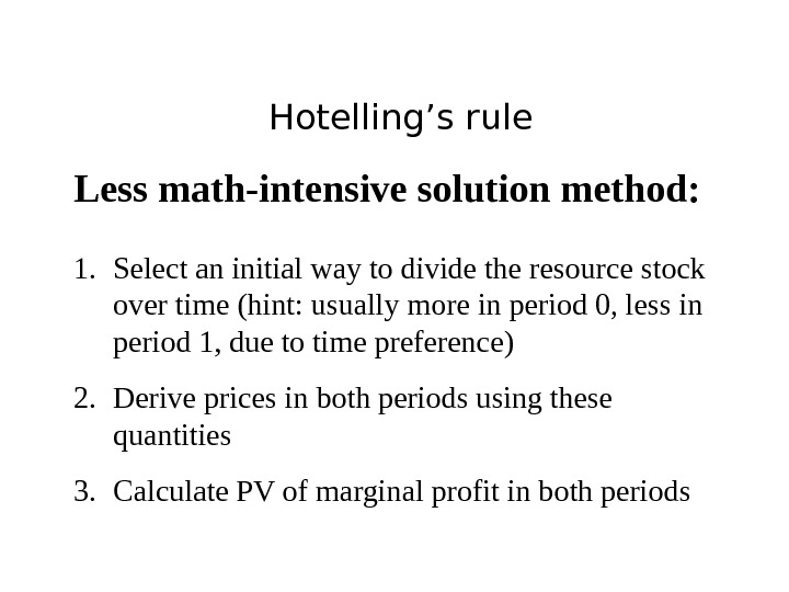
Hotelling’s rule Less math-intensive solution method: 1. Select an initial way to divide the resource stock over time (hint: usually more in period 0, less in period 1, due to time preference) 2. Derive prices in both periods using these quantities 3. Calculate PV of marginal profit in both periods

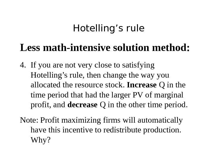
Hotelling’s rule Less math-intensive solution method: 4. If you are not very close to satisfying Hotelling’s rule, then change the way you allocated the resource stock. Increase Q in the time period that had the larger PV of marginal profit, and decrease Q in the other time period. Note: Profit maximizing firms will automatically have this incentive to redistribute production. Why?

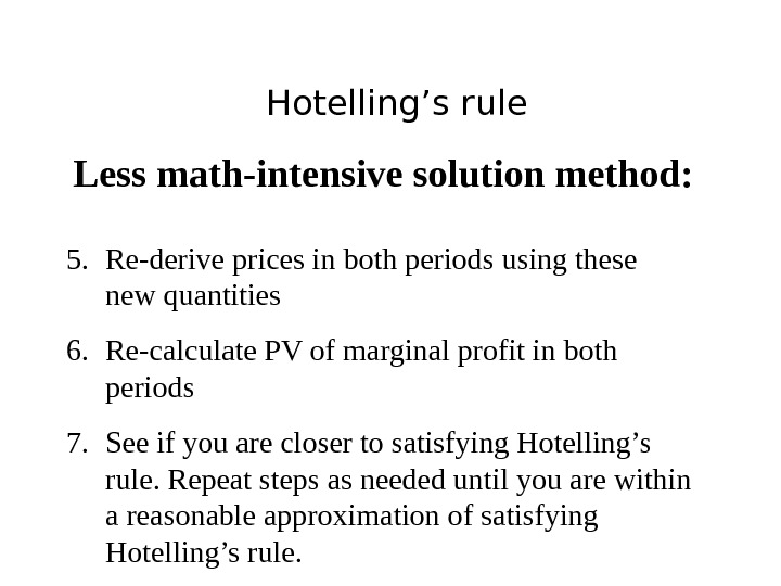
Hotelling’s rule Less math-intensive solution method: 5. Re-derive prices in both periods using these new quantities 6. Re-calculate PV of marginal profit in both periods 7. See if you are closer to satisfying Hotelling’s rule. Repeat steps as needed until you are within a reasonable approximation of satisfying Hotelling’s rule.

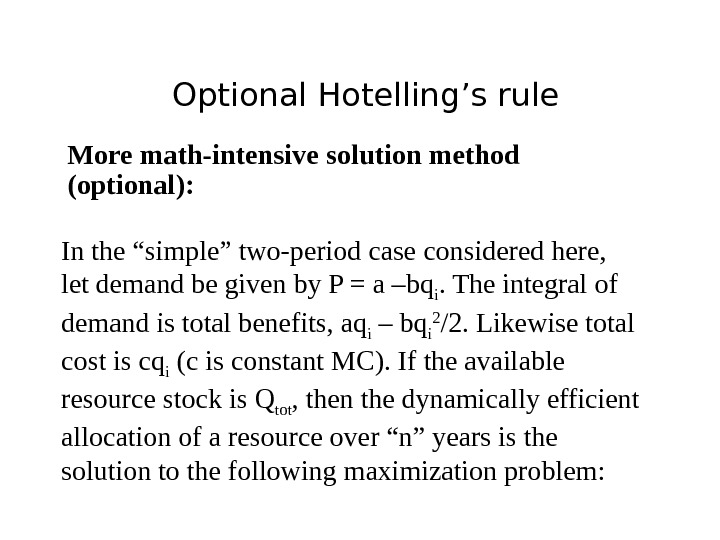
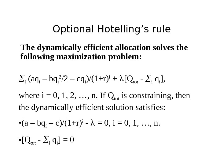
Optional Hotelling’s rule More math-intensive solution method (optional): In the “simple” two-period case considered here, let demand be given by P = a –bq i. The integral of demand is total benefits, aq i – bq i 2 /2. Likewise total cost is cq i (c is constant MC). If the available resource stock is Q tot , then the dynamically efficient allocation of a resource over “n” years is the solution to the following maximization problem:

Optional Hotelling’s rule The dynamically efficient allocation solves the following maximization problem: i (aq i – bq i 2 /2 – cq i )/(1+r) i + [Q tot — i q i ], where i = 0, 1, 2, …, n. If Q tot is constraining, then the dynamically efficient solution satisfies: • (a – bq i – c)/(1+r) i — = 0, i = 0, 1, …, n. • [Q tot — i q i ] =

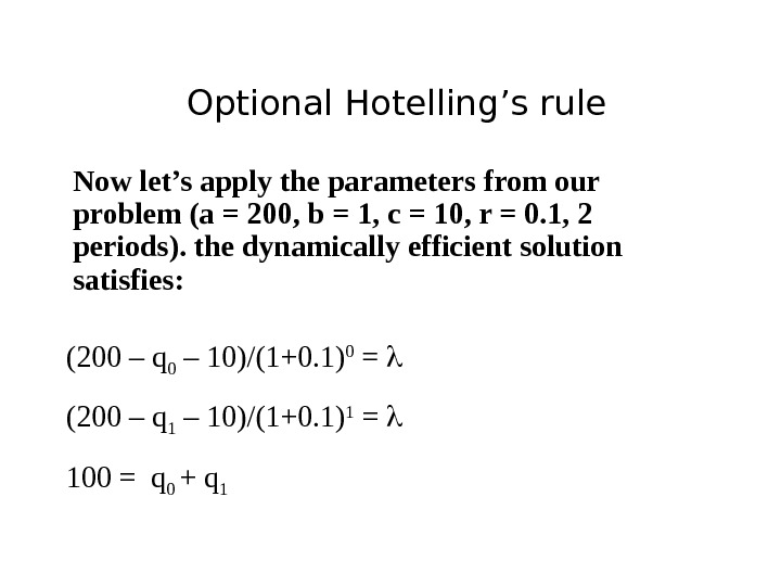
Optional Hotelling’s rule Now let’s apply the parameters from our problem (a = 200, b = 1, c = 10, r = 0. 1, 2 periods). the dynamically efficient solution satisfies: (200 – q 0 – 10)/(1+0. 1) 0 = (200 – q 1 – 10)/(1+0. 1) 1 = 100 = q 0 + q

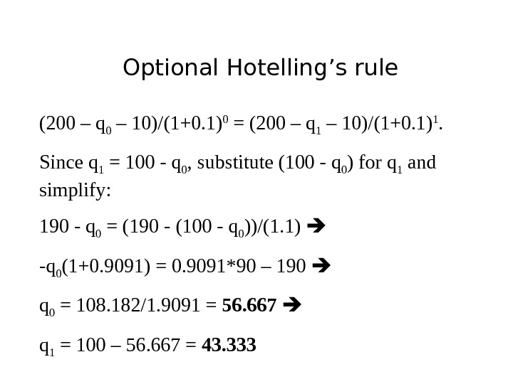
Optional Hotelling’s rule (200 – q 0 – 10)/(1+0. 1) 0 = (200 – q 1 – 10)/(1+0. 1) 1. Since q 1 = 100 — q 0 , substitute (100 — q 0 ) for q 1 and simplify: 190 — q 0 = (190 — (100 — q 0 ))/(1. 1) -q 0 (1+0. 9091) = 0. 9091*90 – 190 q 0 = 108. 182/1. 9091 = 56. 667 q 1 = 100 – 56. 667 = 43.

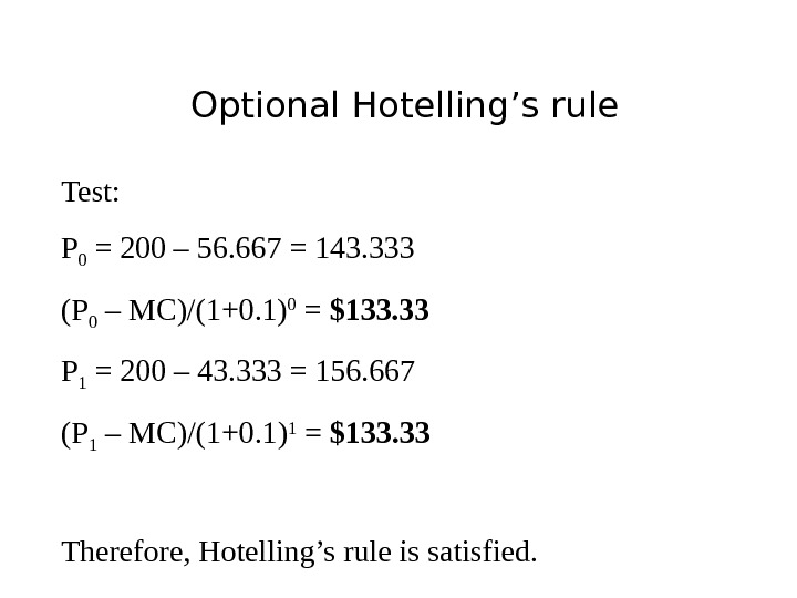
Optional Hotelling’s rule Test: P 0 = 200 – 56. 667 = 143. 333 (P 0 – MC)/(1+0. 1) 0 = $133. 33 P 1 = 200 – 43. 333 = 156. 667 (P 1 – MC)/(1+0. 1) 1 = $133. 33 Therefore, Hotelling’s rule is satisfied.

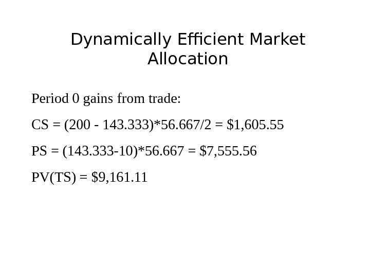
Dynamically Efficient Market Allocation Period 0 gains from trade: CS = (200 — 143. 333)*56. 667/2 = $1, 605. 55 PS = (143. 333 -10)*56. 667 = $7, 555. 56 PV(TS) = $9, 161.

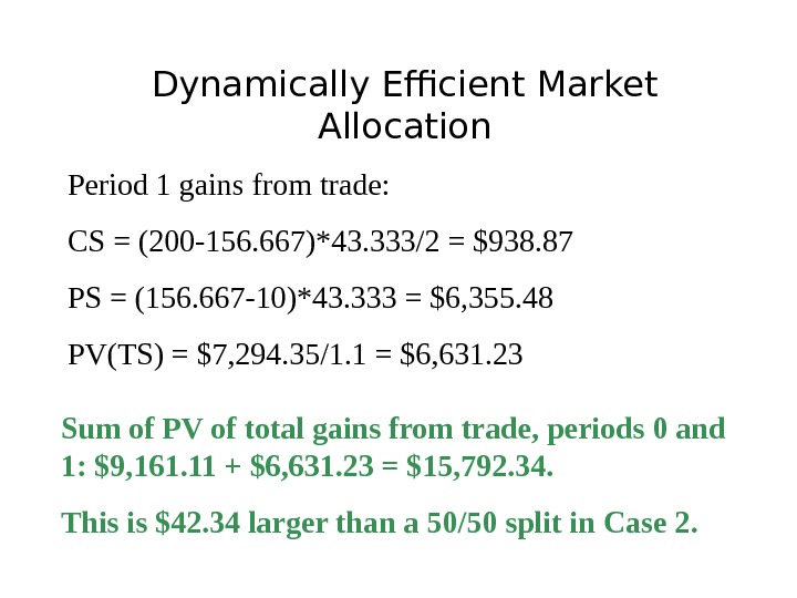
Dynamically Efficient Market Allocation Period 1 gains from trade: CS = (200 -156. 667)*43. 333/2 = $938. 87 PS = (156. 667 -10)*43. 333 = $6, 355. 48 PV(TS) = $7, 294. 35/1. 1 = $6, 631. 23 Sum of PV of total gains from trade, periods 0 and 1: $9, 161. 11 + $6, 631. 23 = $15, 792. 34. This is $42. 34 larger than a 50/50 split in Case 2.

Dynamically efficient equilibrium Intuition If the PV of marginal profit is equal across time periods (Hotelling’s rule), then firms have no incentive to re-arrange production over time. This solution also generates the largest PV of total gains from trade over time.

Dynamically efficient equilibrium Intuition When a resource is abundant then consumption today does not involve an opportunity cost of foregone marginal profit in the future, since there is plenty available for both today and the future. Thus, when resources traded in a competitive market are abundant, P = MC and thus marginal profit is zero. As the resource becomes increasingly scarce , however, consumption today involves an increasingly high opportunity cost of foregone marginal profit in the future. Thus as resources become increasingly scarce relative to demand, marginal profit (P-MC) grows.

Dynamically efficient equilibrium Intuition The profit created by resource scarcity in competitive markets is called Hotelling rent (also known as resource rent or by the Ricardian term scarcity rent ). Hotelling rent is economic profit that can be earned and can persist in certain natural resource cases due to the fixed supply of the resource. Due to fixed supply, consumption of a resource unit today has an opportunity cost equal to the present value of the marginal profit from selling the resource in the future.

Dynamically efficient equilibrium Intuition How will the dynamically efficient allocation of the fixed resource stock change if the discount rate “r” becomes larger? Explain…

Dynamically efficient equilibrium Intuition Suppose that the discount rate remains the same, but the resource stock increases or decreases. How will this affect the dynamically efficient allocation of the resource stock?

Dynamically efficient equilibrium Intuition Under the dynamically efficient solution in our “simplified” modeling framework, what is the trend of price over time? Why?

Dynamically efficient equilibrium Intuition Real world : Natural resource commodity prices may rise or fall over time because: • Marginal production cost might decrease (technology improves) or increase (exploit cheapest sources first). • Demand may grow over time unless a new technology displaces this demand (e. g. , coal replaced firewood, natural gas replaced coal, alt. energy replaces natural gas? ), • Future demand marginal cost cannot be known with certainty.

Dynamically efficient equilibrium Further Study In a graduate natural resources economics class you could evaluate dynamically efficient resource allocation for these more complex and real-world cases: • more than 2 time periods • varying and/or uncertain demand • increasing and/or uncertain marginal cost of production, and • «backstop» technologies allowing for substitutes.

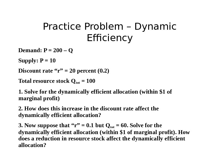
Practice Problem – Dynamic Efficiency Demand: P = 200 – Q Supply: P = 10 Discount rate “r” = 20 percent (0. 2) Total resource stock Q tot = 100 1. Solve for the dynamically efficient allocation (within $1 of marginal profit) 2. How does this increase in the discount rate affect the dynamically efficient allocation? 3. Now suppose that “r” = 0. 1 but Q tot = 60. Solve for the dynamically efficient allocation (within $1 of marginal profit). How does a reduction in resource stock affect the dynamically efficient allocation?