Douglas R White Andrey Korotayev Daria Khaltourina Secular

Douglas R. White Andrey Korotayev Daria Khaltourina Secular Cycles and Millennial Trends Irvine, 2004

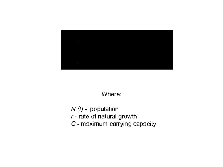Where: N (t) - population r - rate of natural growth C - maximum carrying capacity

Nefedov’s Model of Agrarian Demographic Cycle Q(t) = F[P(t)]A F(P) = Q/A = ksps Q = ksps. A. A(P)= k. P , if k. P< Am A(P)= Am , if k. P > Am AF(Y) = k. Y , if k. Y < Am - AT AF(Y) = Am - AT , if k. Y > Am - AT M = ksq. AF P 0 = p 0 Y(t) W=M+P 0 u = (X (t) – M) /Y (t) Half of the surplus is stored for future consumption: pc = (u+ p 0)/2 if u > p 0 and (u+ p 0)/2 < pm pc = pm if (u+ p 0)/2 > pm If u

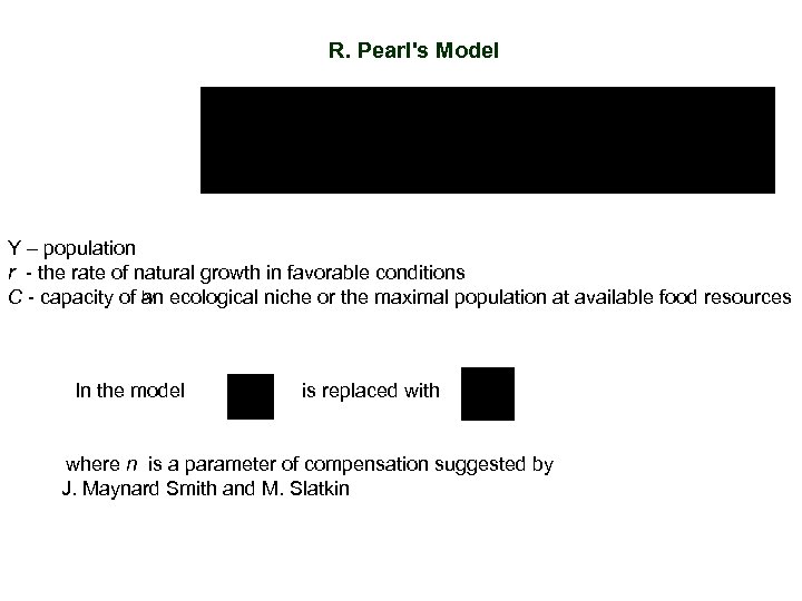R. Pearl's Model Y – population r - the rate of natural growth in favorable conditions by C - capacity of an ecological niche or the maximal population at available food resources In the model is replaced with where n is a parameter of compensation suggested by J. Maynard Smith and M. Slatkin

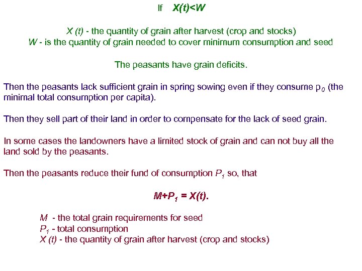If X(t)

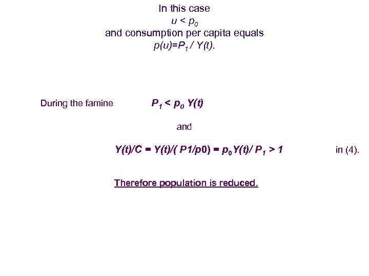In this case u < p 0 and consumption per capita equals p(u)=P 1 / Y(t). During the famine P 1 < p 0 Y(t) and Y(t)/C = Y(t)/( P 1/p 0) = p 0 Y(t)/ P 1 > 1 Therefore population is reduced. in (4).

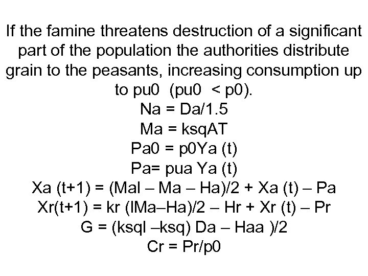If the famine threatens destruction of a significant part of the population the authorities distribute grain to the peasants, increasing consumption up to pu 0 (pu 0 < p 0). Na = Da/1. 5 Ma = ksq. AT Pa 0 = p 0 Ya (t) Pa= pua Ya (t) Xa (t+1) = (Mal – Ma – Ha)/2 + Xa (t) – Pa Xr(t+1) = kr (l. Ma–Ha)/2 – Hr + Xr (t) – Pr G = (ksql –ksq) Da – Haa )/2 Cr = Pr/p 0

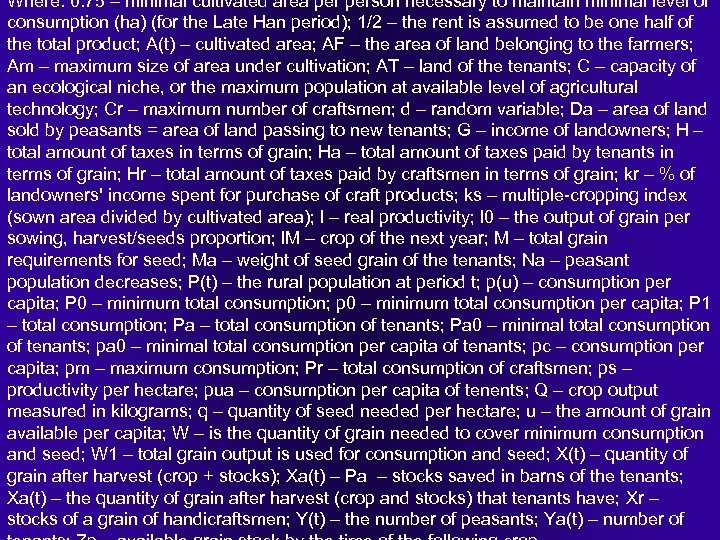Where: 0. 75 – minimal cultivated area person necessary to maintain minimal level of consumption (ha) (for the Late Han period); 1/2 – the rent is assumed to be one half of the total product; A(t) – cultivated area; AF – the area of land belonging to the farmers; Am – maximum size of area under cultivation; AT – land of the tenants; C – capacity of an ecological niche, or the maximum population at available level of agricultural technology; Cr – maximum number of craftsmen; d – random variable; Da – area of land sold by peasants = area of land passing to new tenants; G – income of landowners; H – total amount of taxes in terms of grain; Ha – total amount of taxes paid by tenants in terms of grain; Hr – total amount of taxes paid by craftsmen in terms of grain; kr – % of landowners' income spent for purchase of craft products; ks – multiple-cropping index (sown area divided by cultivated area); l – real productivity; l 0 – the output of grain per sowing, harvest/seeds proportion; l. M – crop of the next year; M – total grain requirements for seed; Ma – weight of seed grain of the tenants; Na – peasant population decreases; P(t) – the rural population at period t; p(u) – consumption per capita; P 0 – minimum total consumption; p 0 – minimum total consumption per capita; P 1 – total consumption; Pa – total consumption of tenants; Pa 0 – minimal total consumption of tenants; pa 0 – minimal total consumption per capita of tenants; pc – consumption per capita; pm – maximum consumption; Pr – total consumption of craftsmen; ps – productivity per hectare; pua – consumption per capita of tenents; Q – crop output measured in kilograms; q – quantity of seed needed per hectare; u – the amount of grain available per capita; W – is the quantity of grain needed to cover minimum consumption and seed; W 1 – total grain output is used for consumption and seed; X(t) – quantity of grain after harvest (crop + stocks); Xa(t) – Pa – stocks saved in barns of the tenants; Xa(t) – the quantity of grain after harvest (crop and stocks) that tenants have; Xr – stocks of a grain of handicraftsmen; Y(t) – the number of peasants; Ya(t) – number of

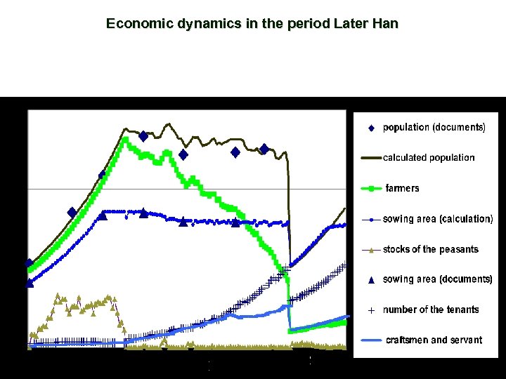Economic dynamics in the period Later Han

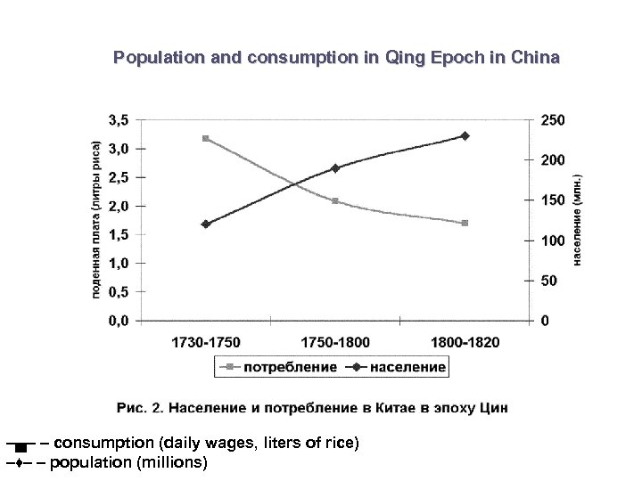Population and consumption in Qing Epoch in China –▄– – consumption (daily wages, liters of rice) –♦– – population (millions)

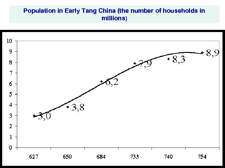Population in Early Tang China (the number of households in millions)

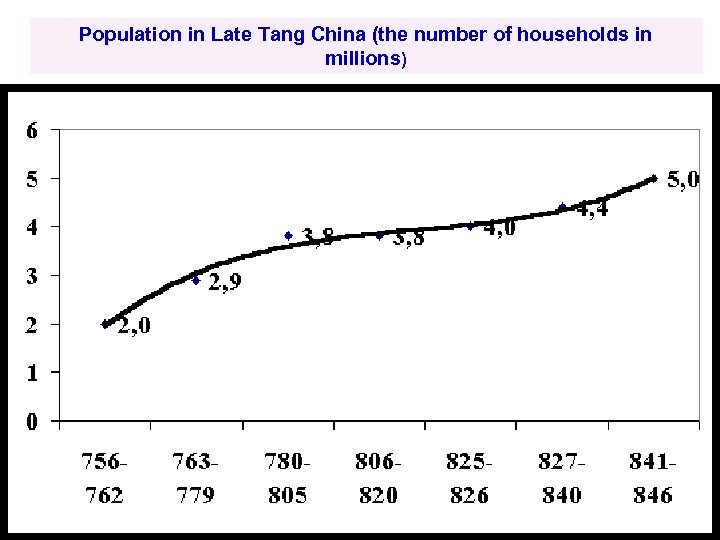Population in Late Tang China (the number of households in millions)

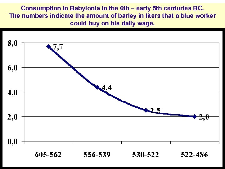Consumption in Babylonia in the 6 th – early 5 th centuries BC. The numbers indicate the amount of barley in liters that a blue worker could buy on his daily wage.

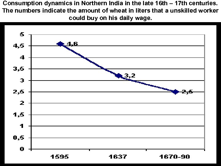Consumption dynamics in Northern India in the late 16 th – 17 th centuries. The numbers indicate the amount of wheat in liters that a unskilled worker could buy on his daily wage.

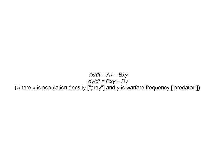dx/dt = Ax – Bxy dy/dt = Cxy – Dy (where x is population density ["prey"] and y is warfare frequency ["predator"])

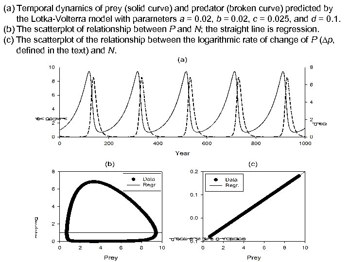(a) Temporal dynamics of prey (solid curve) and predator (broken curve) predicted by the Lotka-Volterra model with parameters a = 0. 02, b = 0. 02, c = 0. 025, and d = 0. 1. (b) The scatterplot of relationship between P and N; the straight line is regression. (c) The scatterplot of the relationship between the logarithmic rate of change of P (∆p, defined in the text) and N.

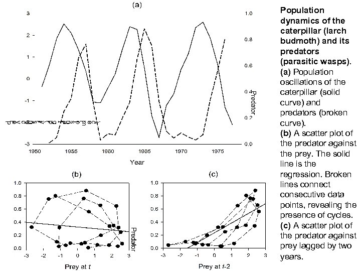Population dynamics of the caterpillar (larch budmoth) and its predators (parasitic wasps). (a) Population oscillations of the caterpillar (solid curve) and predators (broken curve). (b) A scatter plot of the predator against the prey. The solid line is the regression. Broken lines connect consecutive data points, revealing the presence of cycles. (c) A scatter plot of the predator against prey lagged by two years.

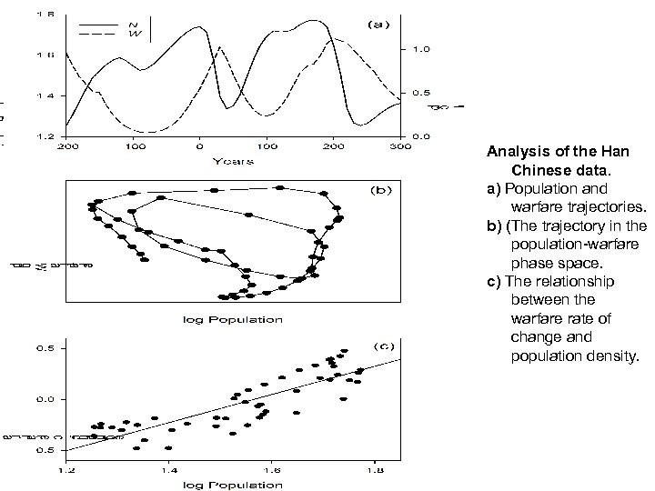Analysis of the Han Chinese data. a) Population and warfare trajectories. b) (The trajectory in the population-warfare phase space. c) The relationship between the warfare rate of change and population density.

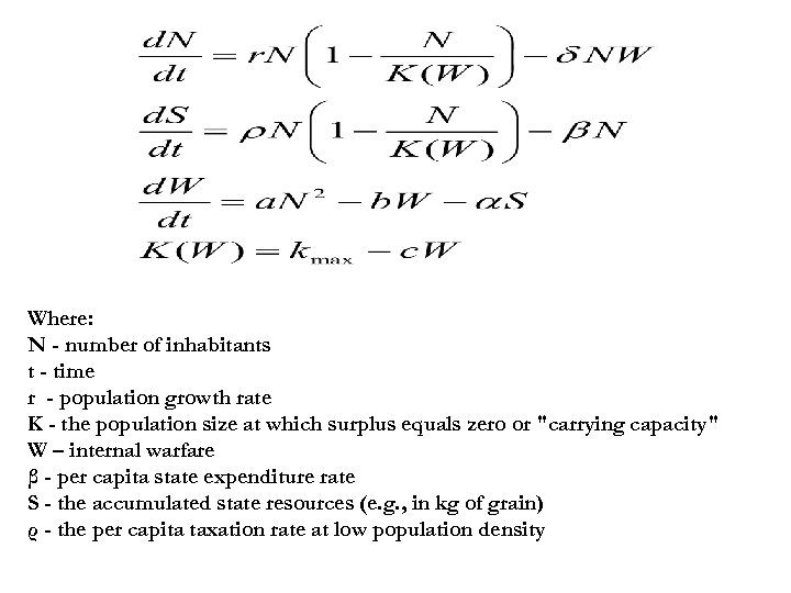Where: N - number of inhabitants t - time r - population growth rate K - the population size at which surplus equals zero or "carrying capacity" W – internal warfare β - per capita state expenditure rate S - the accumulated state resources (e. g. , in kg of grain) ρ - the per capita taxation rate at low population density

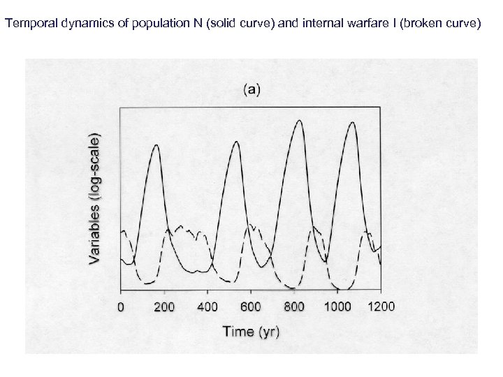Temporal dynamics of population N (solid curve) and internal warfare I (broken curve)

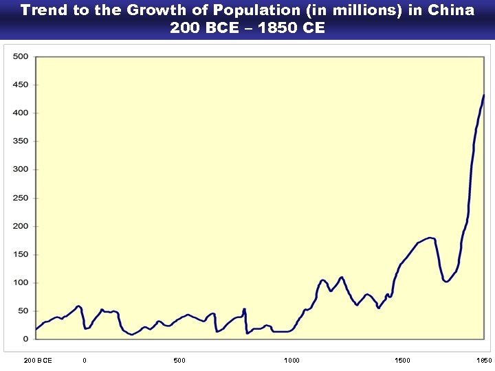Trend to the Growth of Population (in millions) in China 200 BCE – 1850 CE 200 BCE 0 500 1000 1500 1850

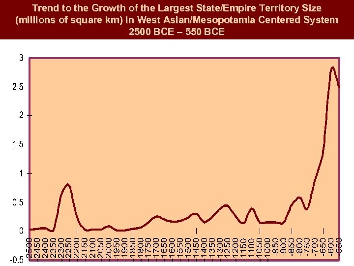Trend to the Growth of the Largest State/Empire Territory Size (millions of square km) in West Asian/Mesopotamia Centered System 2500 BCE – 550 BCE

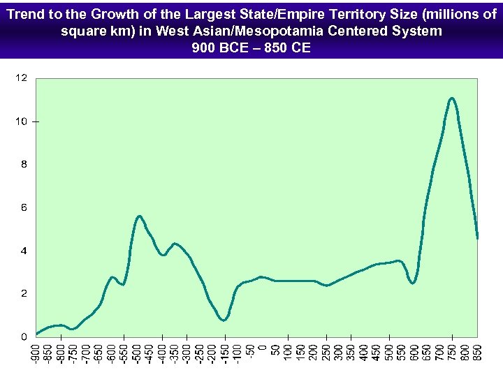Trend to the Growth of the Largest State/Empire Territory Size (millions of square km) in West Asian/Mesopotamia Centered System 900 BCE – 850 CE

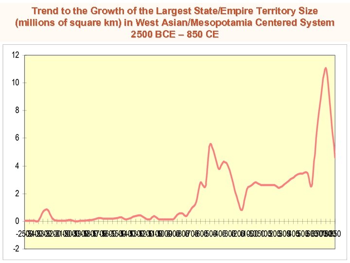Trend to the Growth of the Largest State/Empire Territory Size (millions of square km) in West Asian/Mesopotamia Centered System 2500 BCE – 850 CE

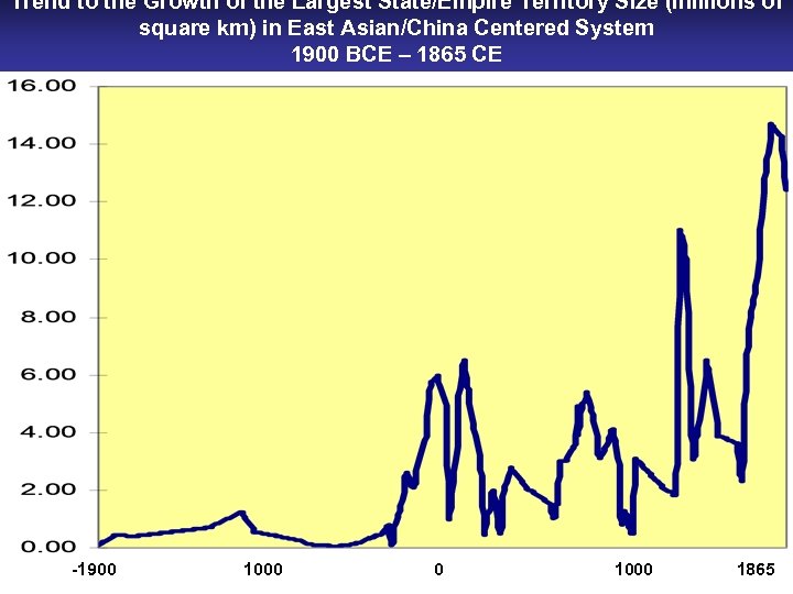Trend to the Growth of the Largest State/Empire Territory Size (millions of square km) in East Asian/China Centered System 1900 BCE – 1865 CE -1900 1000 1865

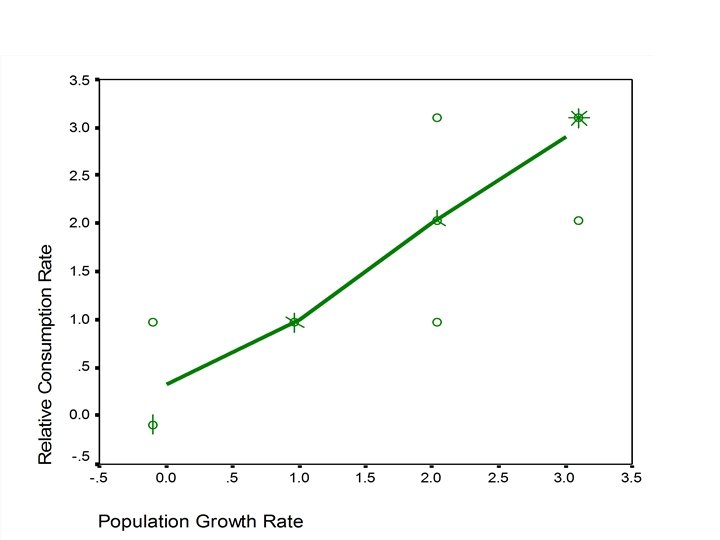
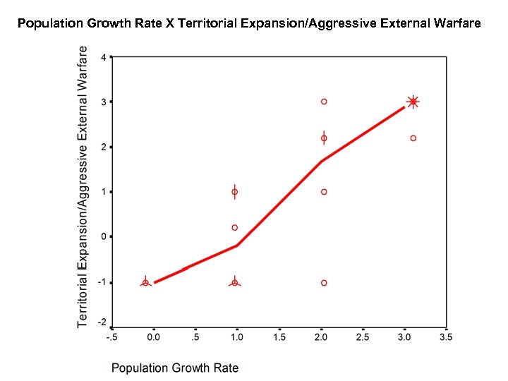Population Growth Rate X Territorial Expansion/Aggressive External Warfare

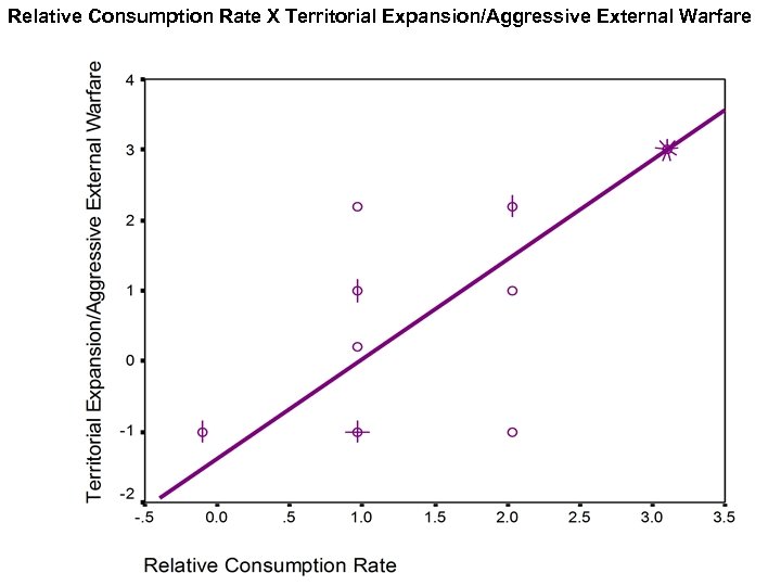Relative Consumption Rate X Territorial Expansion/Aggressive External Warfare

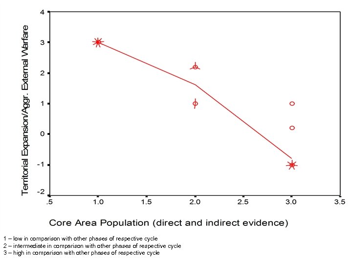1 – low in comparison with other phases of respective cycle 2 – intermediate in comparison with other phases of respective cycle 3 – high in comparison with other phases of respective cycle

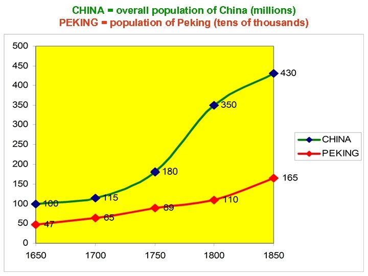CHINA = overall population of China (millions) PEKING = population of Peking (tens of thousands)

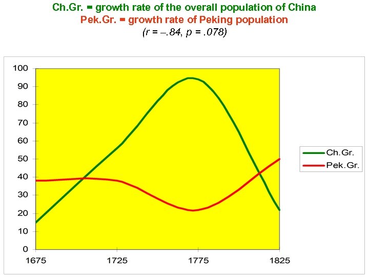Ch. Gr. = growth rate of the overall population of China Pek. Gr. = growth rate of Peking population (r = –. 84, p =. 078)