Domain Adaptation with Multiple Sources Yishay Mansour Tel

Domain Adaptation with Multiple Sources Yishay Mansour, Tel Aviv Univ. & Google Mehryar Mohri, NYU & Google Afshin Rostami, NYU

2

Adaptation – motivation • High level: – The ability to generalize from one domain to another • Significance: – Basic human property – Essential in most learning environments – Implicit in many applications. 3

Adaptation - examples • Sentiment analysis: – Users leave reviews • products, sellers, movies, … – Goal: score reviews as positive or negative. – Adaptation example: • Learn for restaurants and airlines • Generalize to hotels 4

Adaptation - examples • Speech recognition – Adaptation: • Learn a few accents • Generalize to new accents – think “foreign accents”. 5

Adaptation and generalization • Machine Learning prediction: – Learn from examples drawn from distribution D – predict the label of unseen examples • drawn from the same distribution D – generalization within a distribution • Adaptation: – predict the label of unseen examples • drawn from a different distribution D’ – Generalization across distributions 6

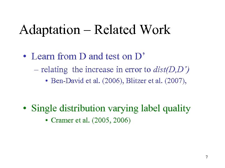Adaptation – Related Work • Learn from D and test on D’ – relating the increase in error to dist(D, D’) • Ben-David et al. (2006), Blitzer et al. (2007), • Single distribution varying label quality • Cramer et al. (2005, 2006) 7

8

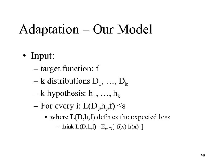
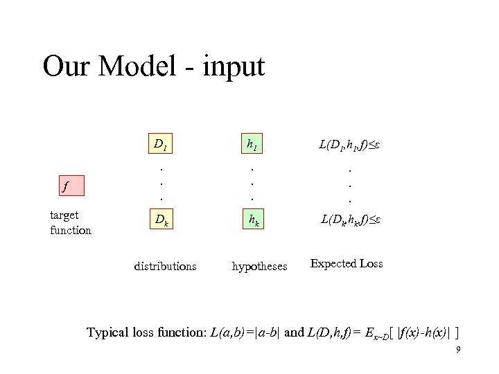Our Model - input D 1 target function L(D 1, h 1, f)≤ε . . . f h 1. . . Dk hk L(Dk, hk, f)≤ε distributions hypotheses Expected Loss Typical loss function: L(a, b)=|a-b| and L(D, h, f)= Ex~D[ |f(x)-h(x)| ] 9

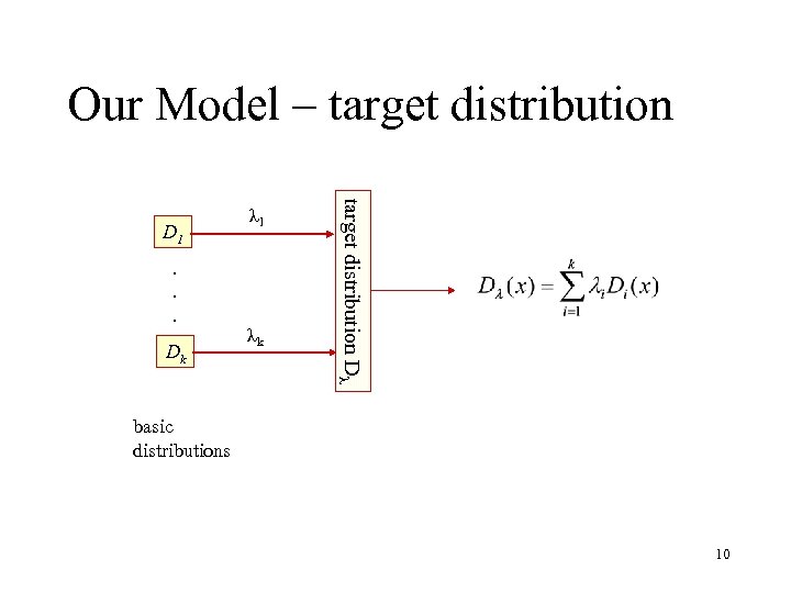Our Model – target distribution . . . Dk λk target distribution Dλ D 1 λ 1 basic distributions 10

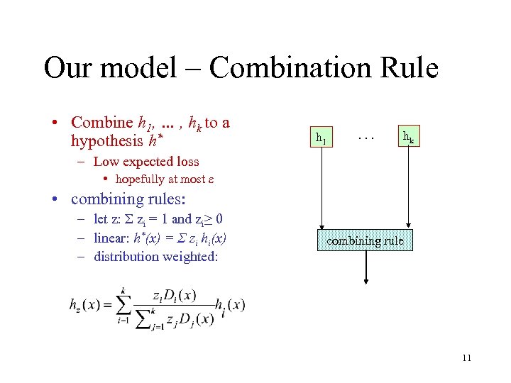Our model – Combination Rule • Combine h 1, … , hk to a hypothesis h* h 1 . . . hk – Low expected loss • hopefully at most ε • combining rules: – let z: Σ zi = 1 and zi≥ 0 – linear: h*(x) = Σ zi hi(x) – distribution weighted: combining rule 11

Combining Rules – Pros • Alternative: Build a dataset for the mixture. – – Learning the mixture parameters is non-trivial Combined data set might be huge size Domain dependent data unavailable Combined data might be huge • Sometimes only classifiers are given/exist – privacy • MOST IMPORTANT: FUNDAMENTAL THEORY QUESTION 12

Our Results: • Linear Combining rule: – Seems like the first thing to try – Can be very bad • Simple settings where any linear combining rule performs badly. 13

Our Results: • Distribution weighted combining rules: – Given the mixture parameter λ: • there is a good distribution weighted combining rule. • expected loss at most ε – For any target function f, • there is a good distribution combining rule hz • expected loss at most ε – Extension for multiple “consistent” target functions • expected loss at most 3ε • OUTCOME: This is the “right” hypothesis class 14

15

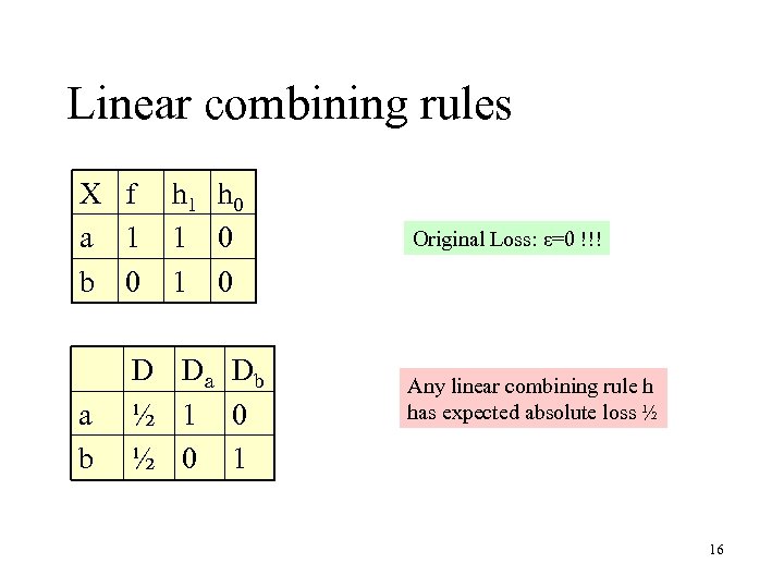Linear combining rules X f a 1 b 0 a b h 1 h 0 1 0 D Da Db ½ 1 0 ½ 0 1 Original Loss: ε=0 !!! Any linear combining rule h has expected absolute loss ½ 16

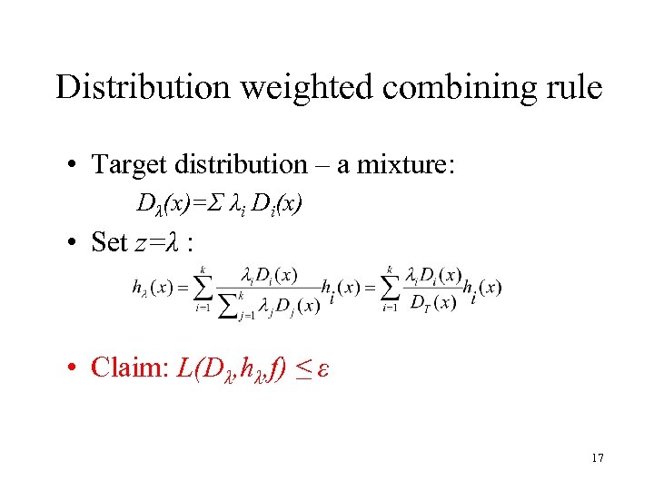Distribution weighted combining rule • Target distribution – a mixture: Dλ(x)=Σ λi Di(x) • Set z=λ : • Claim: L(Dλ, hλ, f) ≤ ε 17

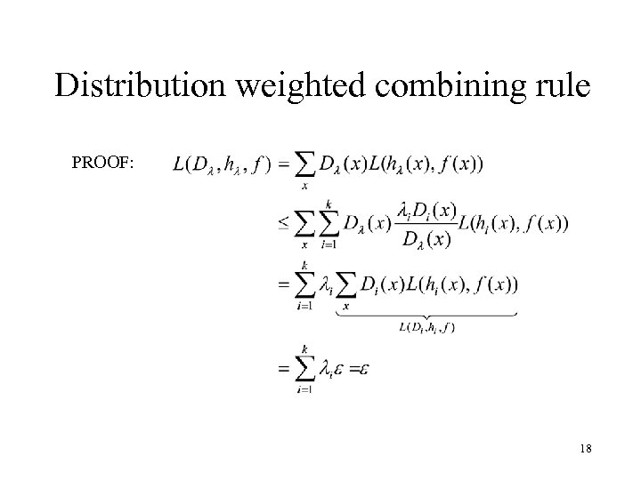Distribution weighted combining rule PROOF: 18

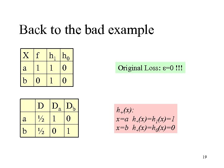Back to the bad example X f a 1 b 0 a b h 1 h 0 1 0 D Da Db ½ 1 0 ½ 0 1 Original Loss: ε=0 !!! h+(x): x=a h+(x)=h 1(x)=1 x=b h+(x)=h 0(x)=0 19

20

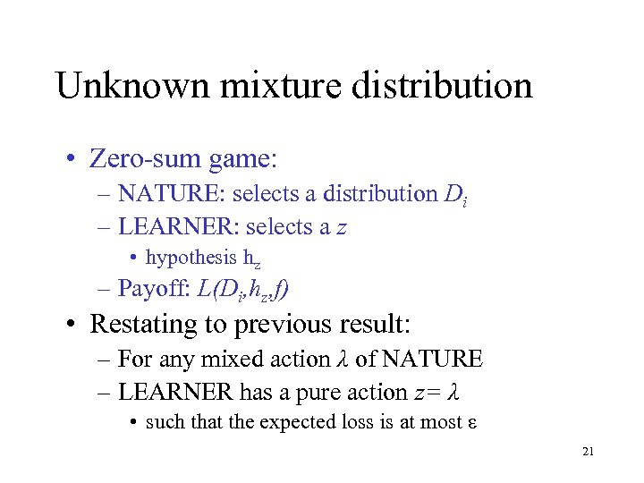Unknown mixture distribution • Zero-sum game: – NATURE: selects a distribution Di – LEARNER: selects a z • hypothesis hz – Payoff: L(Di, hz, f) • Restating to previous result: – For any mixed action λ of NATURE – LEARNER has a pure action z= λ • such that the expected loss is at most ε 21

Unknown mixture distribution • Consequence: – LEARNER has a mixed action (over z’s) – for any mixed action λ of NATURE • a mixture distribution Dλ – The loss is at most ε • Challenge: – show a specific hypothesis hz • pure, not mixed, action 22

Searching for a good hypothesis • Uniformly good hypothesis hz: – for any Di we have L(Di, hz, f) ≤ ε • Assume all the hi are identical – Extremely lucky and unlikely case • If we have a good hypothesis we are done! – L(Dλ, hz, f) = Σ λi L(Di, hz, f) ≤ Σ λi ε = ε • We need to show in general a good hz ! 23

Proof Outline: • Balancing the losses: – Show that some hz has identical loss on any Di – uses Brouwer Fixed Point Theorem • holds very generally • Bounding the losses: – Show this hz has low loss for some mixture • specifically Dz 24

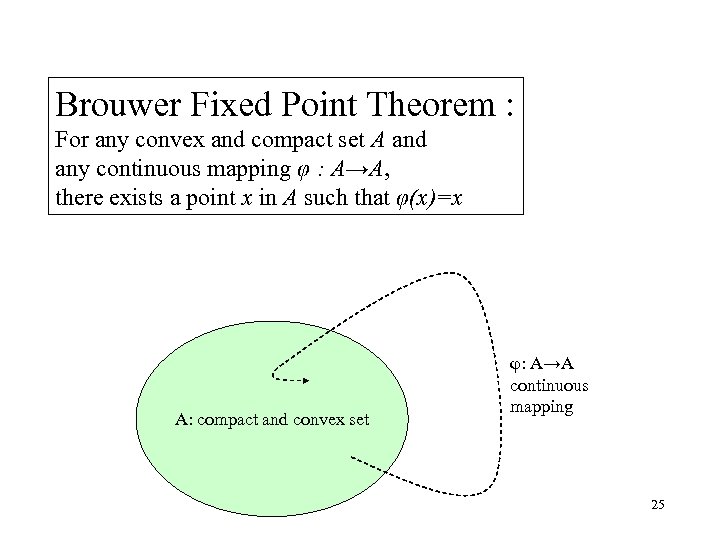Brouwer Fixed Point Theorem : For any convex and compact set A and any continuous mapping φ : A→A, there exists a point x in A such that φ(x)=x A: compact and convex set φ: A→A continuous mapping 25

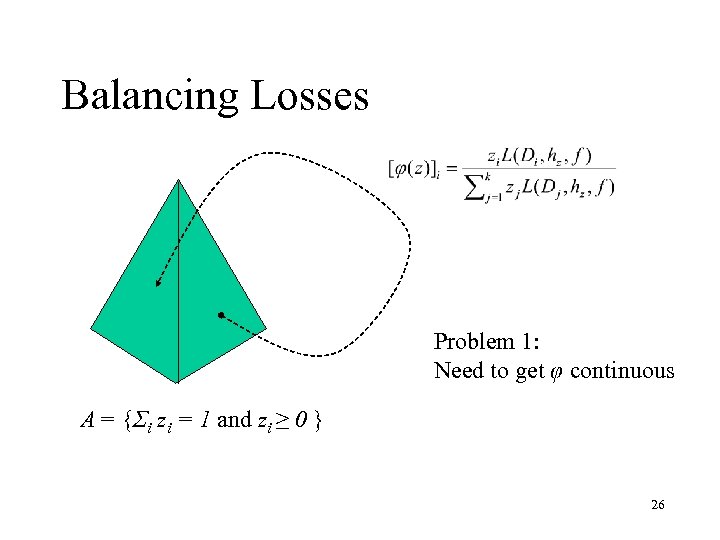Balancing Losses Problem 1: Need to get φ continuous A = {Σi zi = 1 and zi ≥ 0 } 26

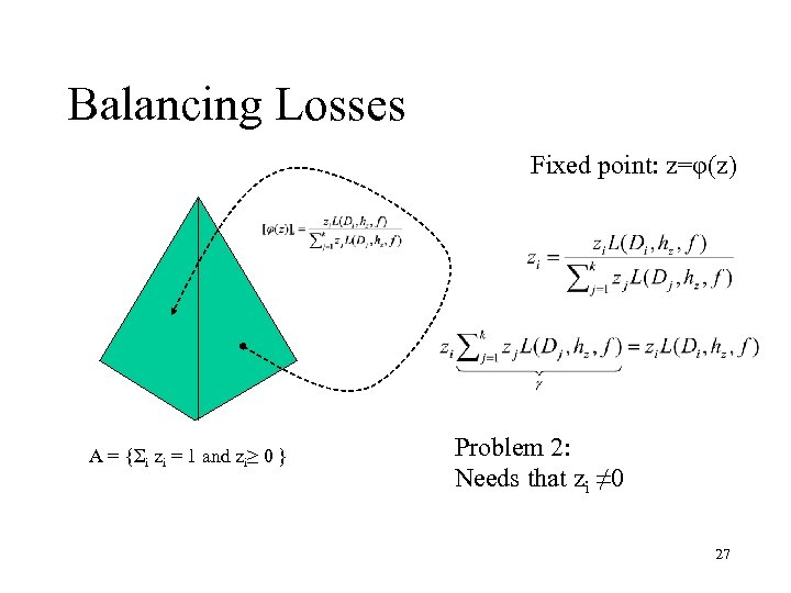Balancing Losses Fixed point: z=φ(z) A = {Σi zi = 1 and zi≥ 0 } Problem 2: Needs that zi ≠ 0 27

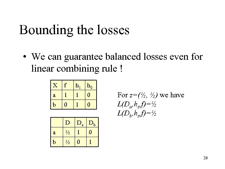Bounding the losses • We can guarantee balanced losses even for linear combining rule ! X f h 1 h 0 a 1 1 0 b 0 1 0 D Da Db a ½ 1 0 b ½ 0 1 For z=(½, ½) we have L(Da, hz, f)=½ L(Db, hz, f)=½ 28

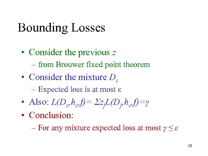Bounding Losses • Consider the previous z – from Brouwer fixed point theorem • Consider the mixture Dz – Expected loss is at most ε • Also: L(Dz, hz, f)= Σzj. L(Dj, hz, f)=γ • Conclusion: – For any mixture expected loss at most γ ≤ ε 29

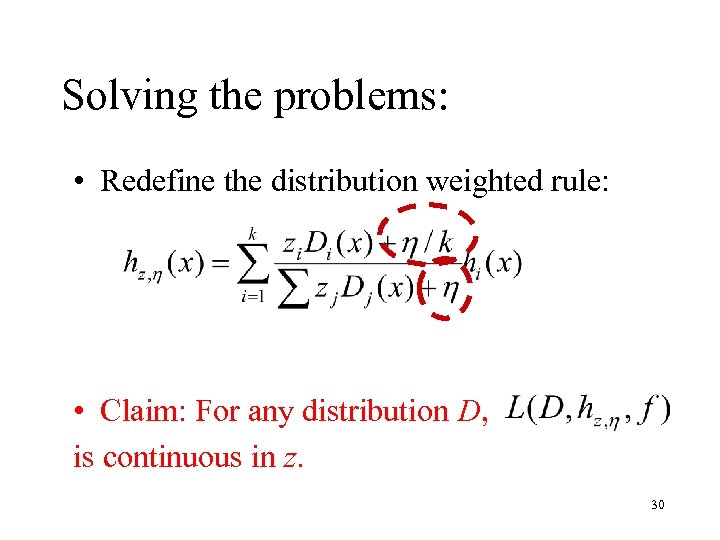Solving the problems: • Redefine the distribution weighted rule: • Claim: For any distribution D, is continuous in z. 30

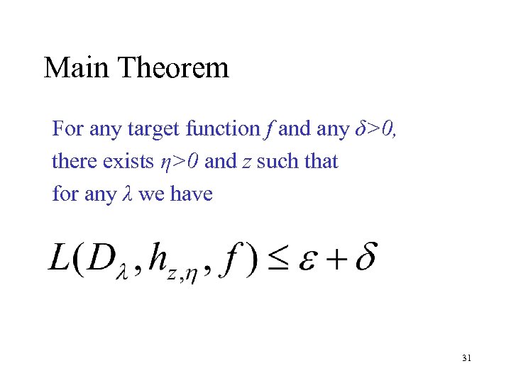Main Theorem For any target function f and any δ>0, there exists η>0 and z such that for any λ we have 31

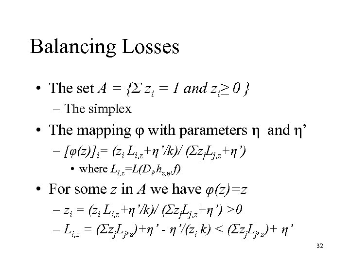Balancing Losses • The set A = {Σ zi = 1 and zi≥ 0 } – The simplex • The mapping φ with parameters η and η’ – [φ(z)]i= (zi Li, z+η’/k)/ (Σzj. Lj, z+η’) • where Li, z=L(Di, hz, η, f) • For some z in A we have φ(z)=z – zi = (zi Li, z+η’/k)/ (Σzj. Lj, z+η’) >0 – Li, z = (Σzj. Lj, z)+η’ - η’/(zi k) < (Σzj. Lj, z)+ η’ 32

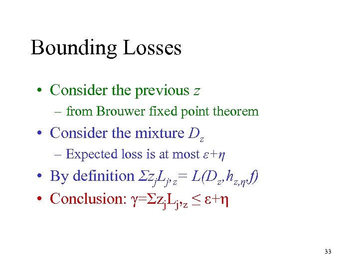Bounding Losses • Consider the previous z – from Brouwer fixed point theorem • Consider the mixture Dz – Expected loss is at most ε+η • By definition Σzj. Lj, z= L(Dz, hz, η, f) • Conclusion: γ=Σzj. Lj, z ≤ ε+η 33

Putting it together • There exists (z, η) such that: – Expected loss of hz, η approximately balanced – L(Di, hz, η, f) ≤γ+η’ • Bounding γ using Dz – γ =L(Dz, hz, η, f) ≤ε+η • For any mixture Dλ – L(Dλ, hz, η, f) ≤ε+η+ η’ 34

A more general model • So far: NATURE first fixes target function f • consistent target functions f – the expected loss w. r. t. Di is at most ε • for any of the k distributions • Function class F ={f is consistent} • New Model: – LEARNER picks a hypothesis h – NATURE picks f in F and mixture Dλ – Loss L(Dλ, h, f) • RESULT: L(Dλ, h, f)≤ 3ε. 35

36

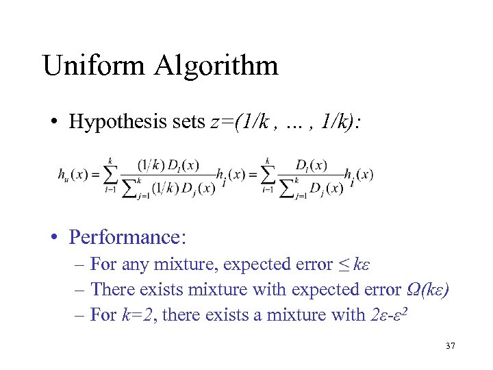Uniform Algorithm • Hypothesis sets z=(1/k , … , 1/k): • Performance: – For any mixture, expected error ≤ kε – There exists mixture with expected error Ω(kε) – For k=2, there exists a mixture with 2ε-ε 2 37

Open Problem • Find a uniformly good hypothesis – efficiently !!! • algorithmic issues: – Search over the z’s – Multiple local minima. 38

39

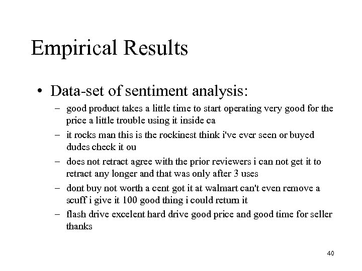Empirical Results • Data-set of sentiment analysis: – good product takes a little time to start operating very good for the price a little trouble using it inside ca – it rocks man this is the rockinest think i've ever seen or buyed dudes check it ou – does not retract agree with the prior reviewers i can not get it to retract any longer and that was only after 3 uses – dont buy not worth a cent got it at walmart can't even remove a scuff i give it 100 good thing i could return it – flash drive excelent hard drive good price and good time for seller thanks 40

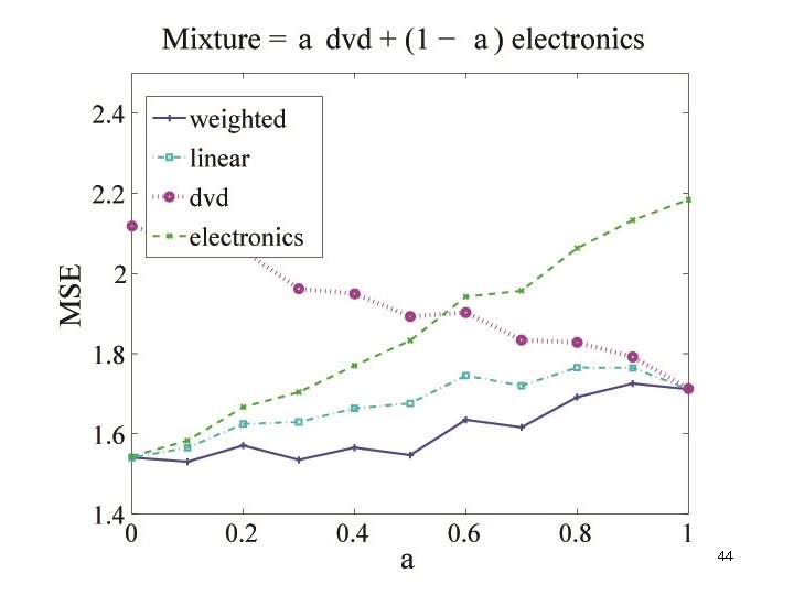
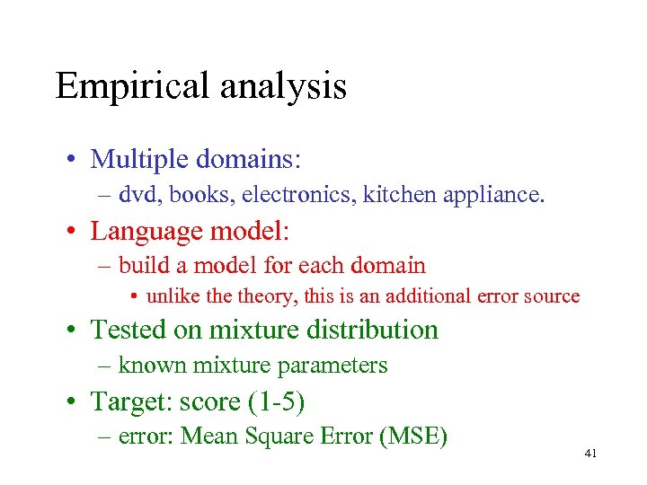Empirical analysis • Multiple domains: – dvd, books, electronics, kitchen appliance. • Language model: – build a model for each domain • unlike theory, this is an additional error source • Tested on mixture distribution – known mixture parameters • Target: score (1 -5) – error: Mean Square Error (MSE) 41

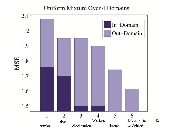books dvd kitchen electronics linear Distribution weighted 42

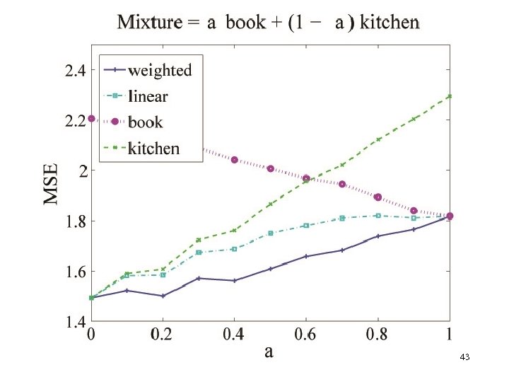43

44

45

Summary • Adaptation model – combining rules • linear • distribution weighted • Theoretical analysis – mixture distribution • Future research – algorithms for combining rules – beyond mixtures 46

47

Adaptation – Our Model • Input: – target function: f – k distributions D 1, …, Dk – k hypothesis: h 1, …, hk – For every i: L(Di, hi, f) ≤ε • where L(D, h, f) defines the expected loss – think L(D, h, f)= Ex~D[ |f(x)-h(x)| ] 48