DOE Design Analysis Using Minitab L Goch

DOE Design & Analysis Using Minitab L. Goch – February 2011

AGENDA DOE Design DOE Pitfalls & Types of Designs Screen Design Example Characterization Design Example Optimization Design Example DOE Analysis Response Surface Design

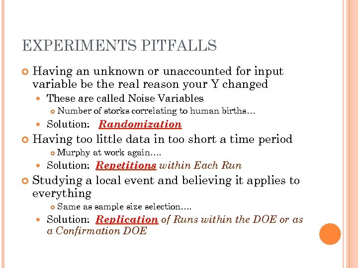
EXPERIMENTS PITFALLS Having an unknown or unaccounted for input variable be the real reason your Y changed These are called Noise Variables Solution: Randomization Having too little data in too short a time period Number of storks correlating to human births… Murphy at work again…. Solution: Repetitions within Each Run Studying a local event and believing it applies to everything Same as sample size selection…. Solution: Replication of Runs within the DOE or as a Confirmation DOE

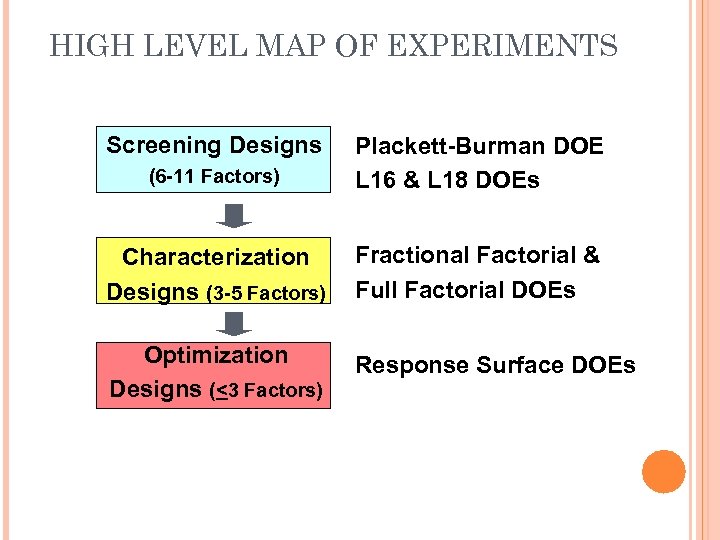
HIGH LEVEL MAP OF EXPERIMENTS Screening Designs (6 -11 Factors) Plackett-Burman DOE L 16 & L 18 DOEs Characterization Designs (3 -5 Factors) Fractional Factorial & Full Factorial DOEs Optimization Designs (<3 Factors) Response Surface DOEs

SCREENING DESIGNS v PLACKETT-BURMAN EXAMPLE (2 LEVEL DOE) üSTAT > DOE > FACTORIAL > CREATE FACTORIAL DESIGN üCHECK ‘PLACKETT-BURMAN DESIGN’ ü WILL REVIEW DURING TRAINING v L 16 & L 18 ARE ALSO GOOD SCREENING DESIGNS (2 & 3 LEVEL MIXED DOE) üSTAT > DOE > TAGUCHI > CREATE TAGUCHI DESIGN üCHECK ‘MIXED LEVEL DESIGN’ üREVIEW ON OWN

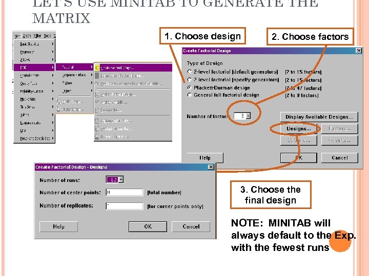
LET’S USE MINITAB TO GENERATE THE MATRIX 1. Choose design 2. Choose factors 3. Choose the final design NOTE: MINITAB will always default to the Exp. with the fewest runs

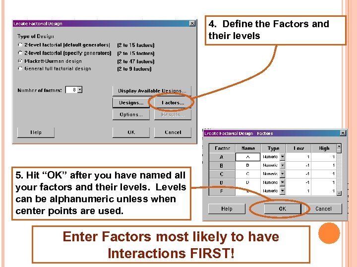
DESIGN MATRIX 4. Define the Factors and their levels 5. Hit “OK” after you have named all your factors and their levels. Levels can be alphanumeric unless when center points are used. Enter Factors most likely to have Interactions FIRST!

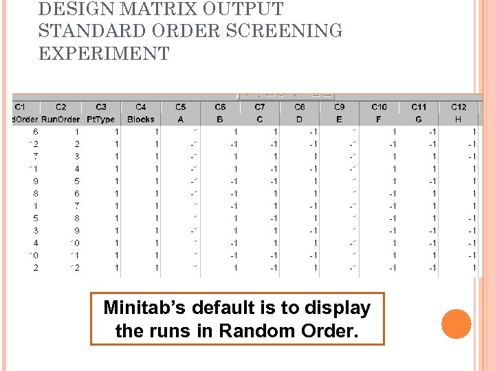
DESIGN MATRIX OUTPUT STANDARD ORDER SCREENING EXPERIMENT Minitab’s default is to display the runs in Random Order.

CHARACTERIZATION DESIGNS v FULL FACTORIAL DOE üSTAT > DOE > FACTORIAL > CREATE FACTORIAL DESIGN üCHECK ‘GENERAL FULL FACTORIAL DESIGN’ ü REVIEW ON OWN v FRACTIONAL FACTORIAL DOE üSTAT > DOE > FACTORIAL > CREATE FACTORIAL DESIGN üCHECK ‘ 2 -LEVEL FACTORIAL (DEFAULT GENERATORS)’ üWILL REVIEW DURING TRAINING

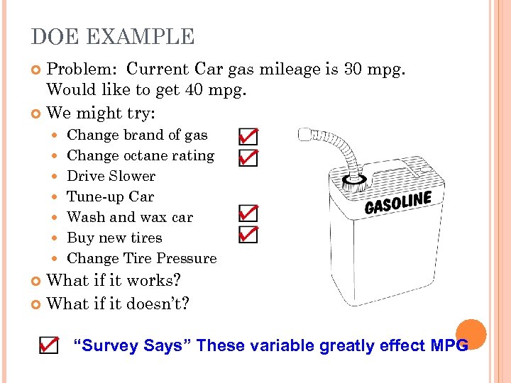
DOE EXAMPLE Problem: Current Car gas mileage is 30 mpg. Would like to get 40 mpg. We might try: Change brand of gas Change octane rating Drive Slower Tune-up Car Wash and wax car Buy new tires Change Tire Pressure What if it works? What if it doesn’t? “Survey Says” These variable greatly effect MPG

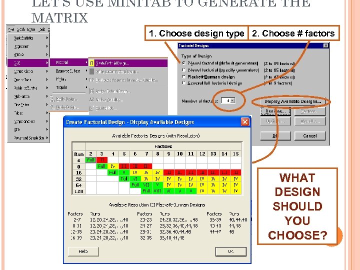
LET’S USE MINITAB TO GENERATE THE MATRIX 1. Choose design type 2. Choose # factors WHAT DESIGN SHOULD YOU CHOOSE?

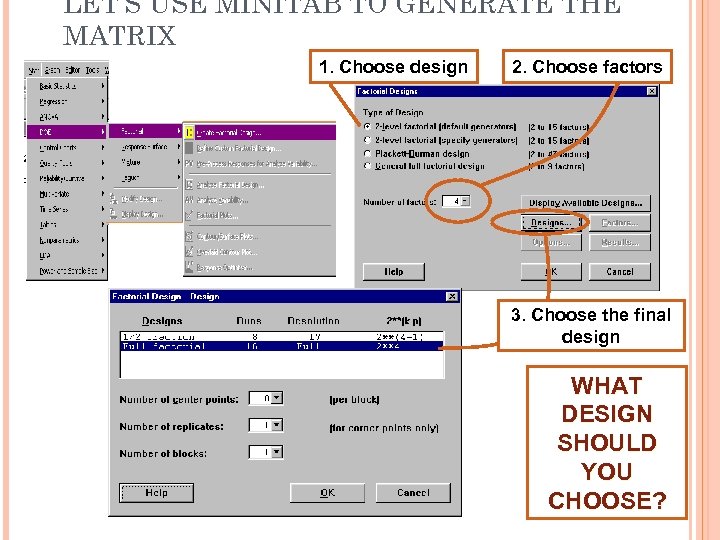
LET’S USE MINITAB TO GENERATE THE MATRIX 1. Choose design 2. Choose factors 3. Choose the final design WHAT DESIGN SHOULD YOU CHOOSE?

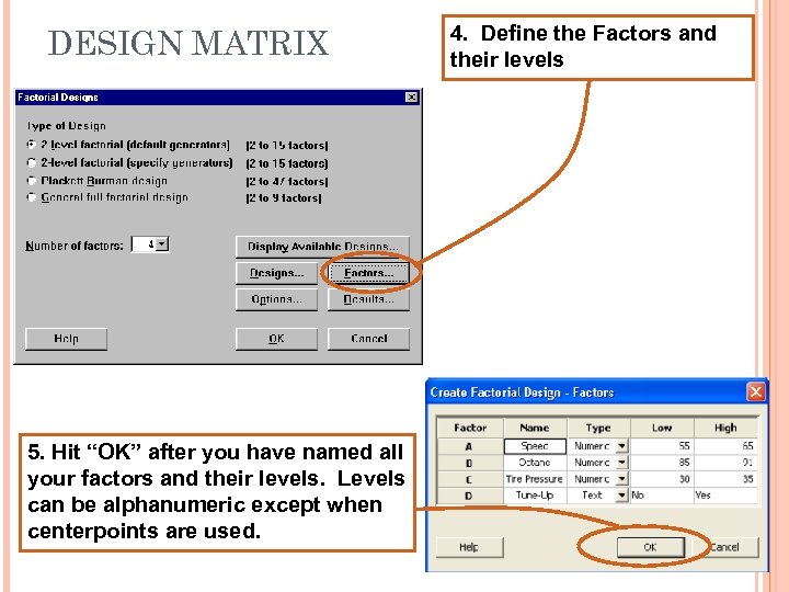
DESIGN MATRIX 5. Hit “OK” after you have named all your factors and their levels. Levels can be alphanumeric except when centerpoints are used. 4. Define the Factors and their levels

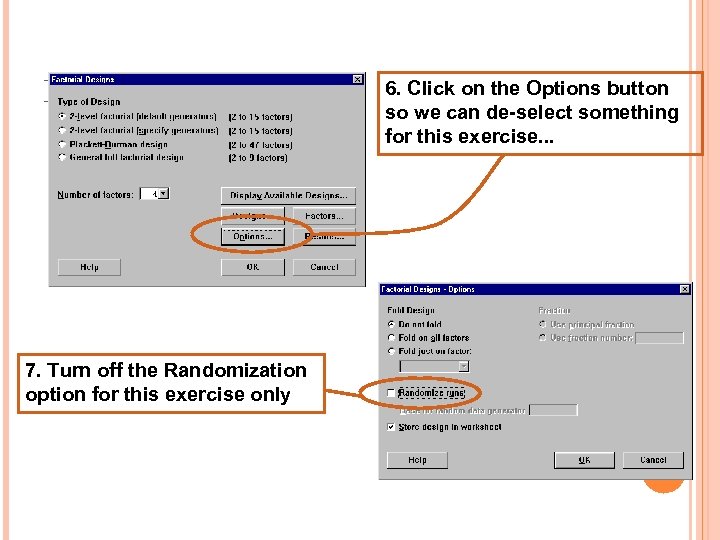
DESIGN MATRIX 7. Turn off the Randomization option for this exercise only 6. Click on the Options button so we can de-select something for this exercise. . .

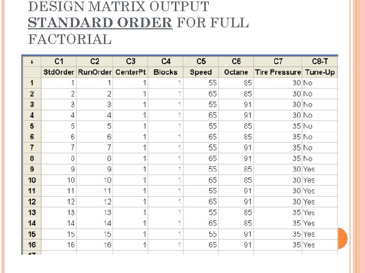
DESIGN MATRIX OUTPUT STANDARD ORDER FOR FULL FACTORIAL

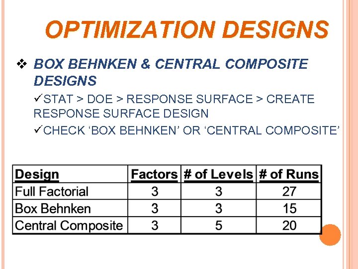
OPTIMIZATION DESIGNS v BOX BEHNKEN & CENTRAL COMPOSITE DESIGNS üSTAT > DOE > RESPONSE SURFACE > CREATE RESPONSE SURFACE DESIGN üCHECK ‘BOX BEHNKEN’ OR ‘CENTRAL COMPOSITE’

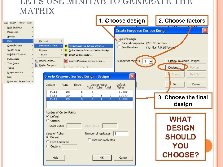
LET’S USE MINITAB TO GENERATE THE MATRIX 1. Choose design 2. Choose factors 3. Choose the final design WHAT DESIGN SHOULD YOU CHOOSE?

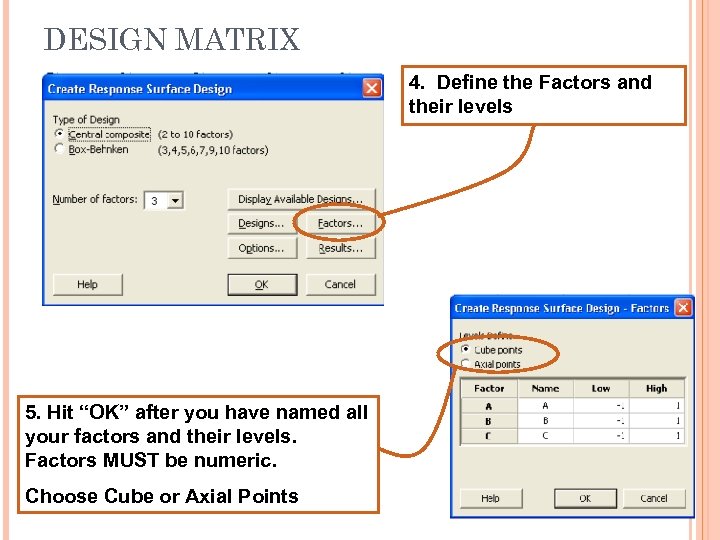
DESIGN MATRIX 4. Define the Factors and their levels 5. Hit “OK” after you have named all your factors and their levels. Factors MUST be numeric. Choose Cube or Axial Points

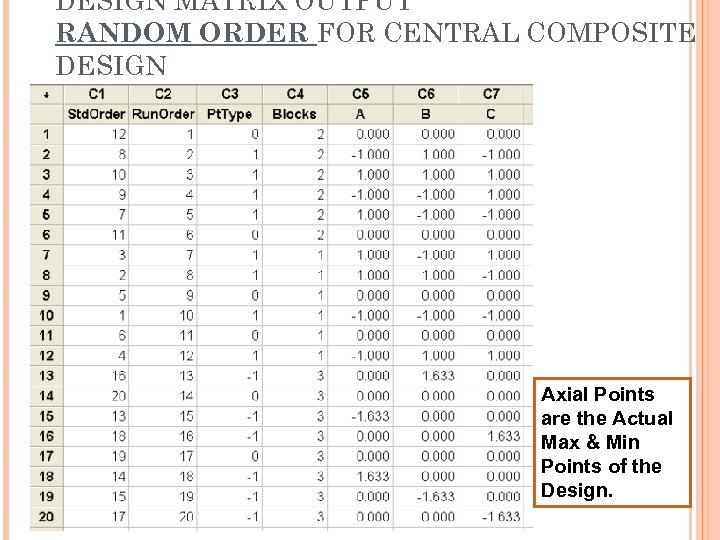
DESIGN MATRIX OUTPUT RANDOM ORDER FOR CENTRAL COMPOSITE DESIGN Axial Points are the Actual Max & Min Points of the Design.

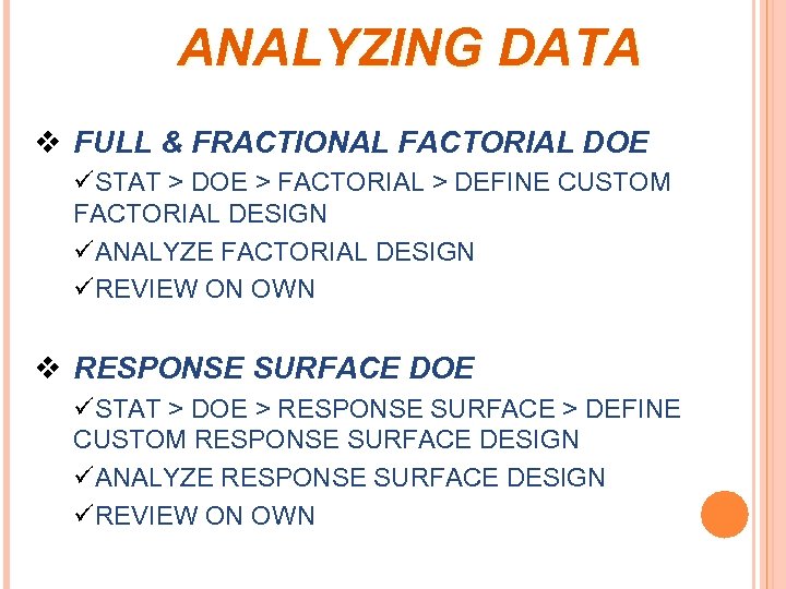
ANALYZING DATA v FULL & FRACTIONAL FACTORIAL DOE üSTAT > DOE > FACTORIAL > DEFINE CUSTOM FACTORIAL DESIGN üANALYZE FACTORIAL DESIGN üREVIEW ON OWN v RESPONSE SURFACE DOE üSTAT > DOE > RESPONSE SURFACE > DEFINE CUSTOM RESPONSE SURFACE DESIGN üANALYZE RESPONSE SURFACE DESIGN üREVIEW ON OWN

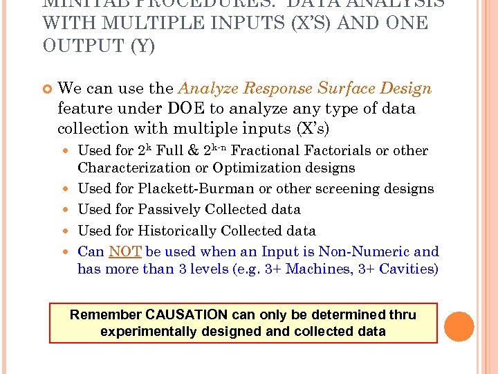
MINITAB PROCEDURES: DATA ANALYSIS WITH MULTIPLE INPUTS (X’S) AND ONE OUTPUT (Y) We can use the Analyze Response Surface Design feature under DOE to analyze any type of data collection with multiple inputs (X’s) Used for 2 k Full & 2 k-n Fractional Factorials or other Characterization or Optimization designs Used for Plackett-Burman or other screening designs Used for Passively Collected data Used for Historically Collected data Can NOT be used when an Input is Non-Numeric and has more than 3 levels (e. g. 3+ Machines, 3+ Cavities) Remember CAUSATION can only be determined thru experimentally designed and collected data

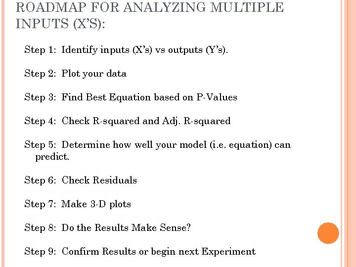
ROADMAP FOR ANALYZING MULTIPLE INPUTS (X’S): Step 1: Step 2: Step 3: Step 4: Identify inputs (X’s) vs outputs (Y’s). Plot your data Find Best Equation based on P-Values Check R-squared and Adj. R-squared Step 5: Determine how well your model (i. e. equation) can predict. Step 6: Step 7: Step 8: Step 9: Check Residuals Make 3 -D plots Do the Results Make Sense? Confirm Results or begin next Experiment

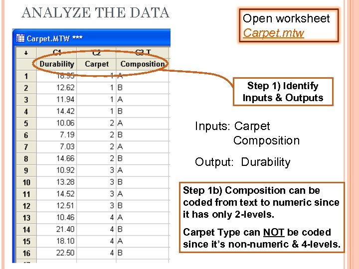
ANALYZE THE DATA Open worksheet Carpet. mtw Step 1) Identify Inputs & Outputs Inputs: Carpet Composition Output: Durability Step 1 b) Composition can be coded from text to numeric since it has only 2 -levels. Carpet Type can NOT be coded since it’s non-numeric & 4 -levels.

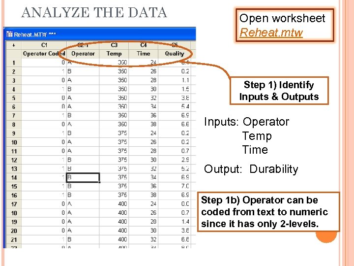
ANALYZE THE DATA Open worksheet Reheat. mtw Step 1) Identify Inputs & Outputs Inputs: Operator Temp Time Output: Durability Step 1 b) Operator can be coded from text to numeric since it has only 2 -levels.

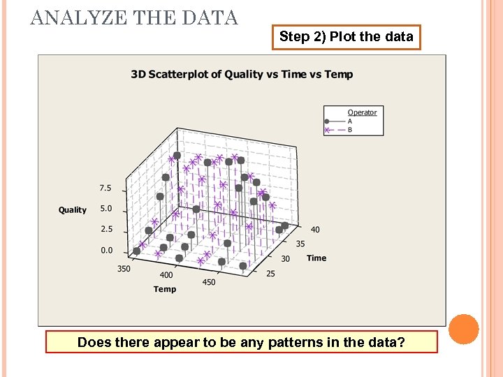
ANALYZE THE DATA Step 2) Plot the data Does there appear to be any patterns in the data?

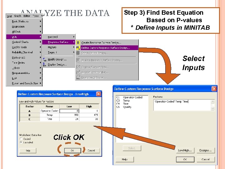
ANALYZE THE DATA Step 3) Find Best Equation Based on P-values * Define Inputs in MINITAB Select Inputs Click OK

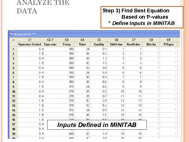
ANALYZE THE DATA Step 3) Find Best Equation Based on P-values * Define Inputs in MINITAB Inputs Defined in MINITAB

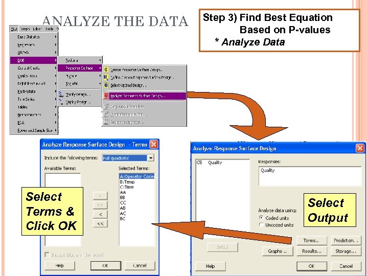
ANALYZE THE DATA Select Terms & Click OK Step 3) Find Best Equation Based on P-values * Analyze Data Select Output

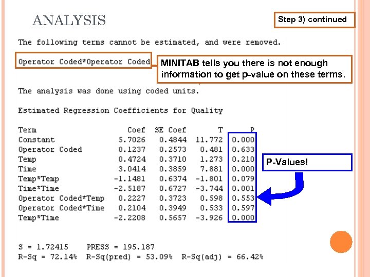
ANALYSIS Step 3) continued MINITAB tells you there is not enough information to get p-value on these terms. P-Values!

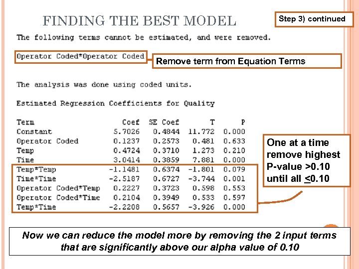
FINDING THE BEST MODEL Step 3) continued Remove term from Equation Terms One at a time remove highest P-value >0. 10 until all <0. 10 Now we can reduce the model more by removing the 2 input terms that are significantly above our alpha value of 0. 10

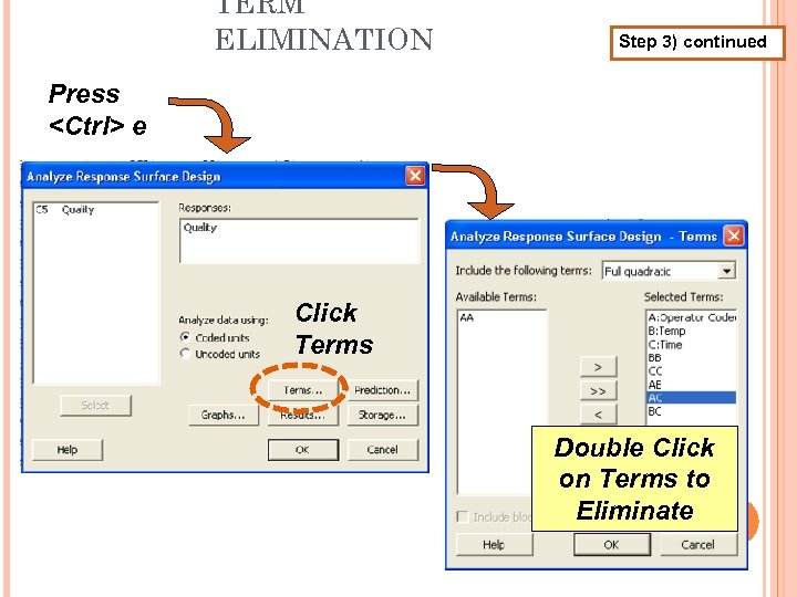
TERM ELIMINATION Step 3) continued Press <Ctrl> e Click Terms Double Click on Terms to Eliminate

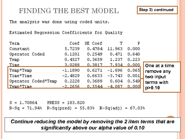
FINDING THE BEST MODEL Step 3) continued One at a time remove any two input terms with p>0. 10 Continue reducing the model by removing the 2 item terms that are significantly above our alpha value of 0. 10

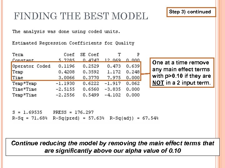
FINDING THE BEST MODEL Step 3) continued One at a time remove any main effect terms with p>0. 10 if they are NOT in a 2 input term. Continue reducing the model by removing the main effect terms that are significantly above our alpha value of 0. 10

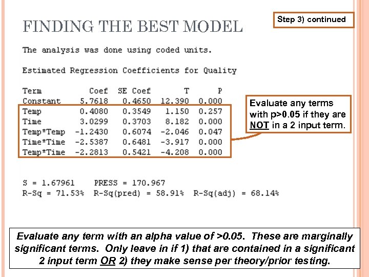
FINDING THE BEST MODEL Step 3) continued Evaluate any terms with p>0. 05 if they are NOT in a 2 input term. Evaluate any term with an alpha value of >0. 05. These are marginally significant terms. Only leave in if 1) that are contained in a significant 2 input term OR 2) they make sense per theory/prior testing.

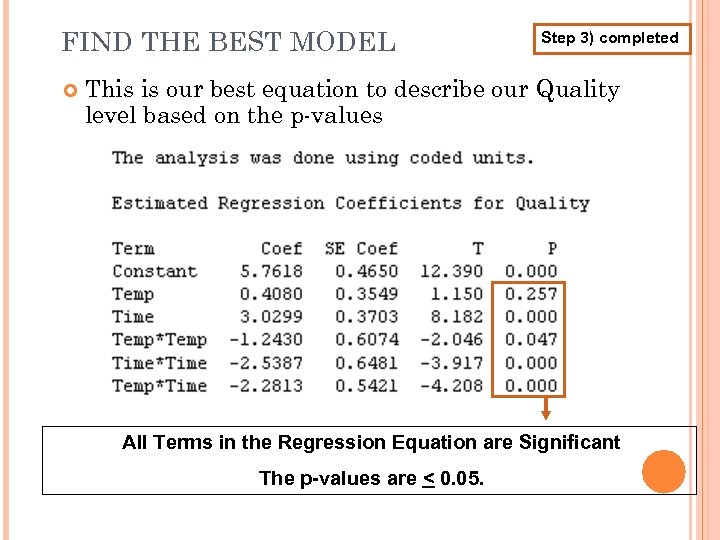
FIND THE BEST MODEL Step 3) completed This is our best equation to describe our Quality level based on the p-values All Terms in the Regression Equation are Significant The p-values are < 0. 05.

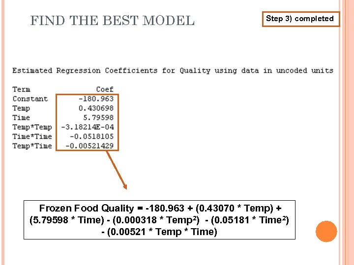
FIND THE BEST MODEL Step 3) completed Frozen Food Quality = -180. 963 + (0. 43070 * Temp) + (5. 79598 * Time) - (0. 000318 * Temp 2) - (0. 05181 * Time 2) - (0. 00521 * Temp * Time)

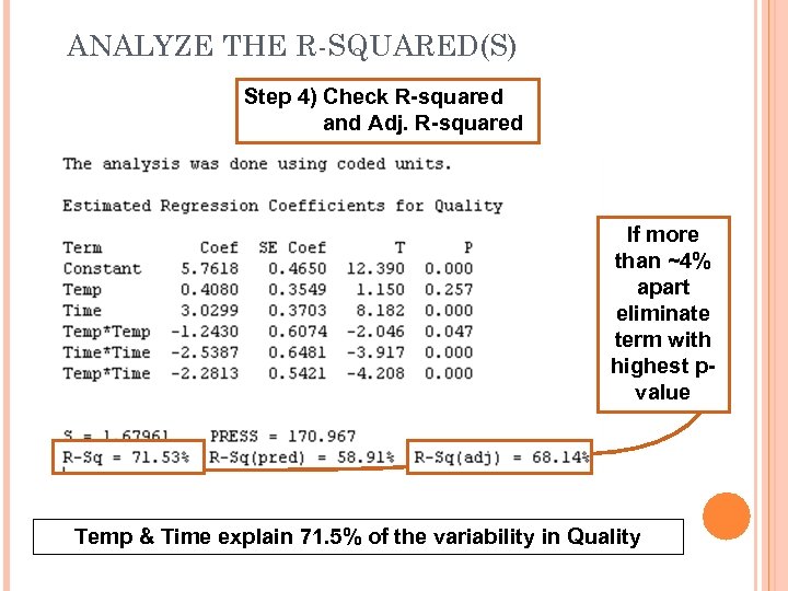
ANALYZE THE R-SQUARED(S) Step 4) Check R-squared and Adj. R-squared If more than ~4% apart eliminate term with highest pvalue Temp & Time explain 71. 5% of the variability in Quality

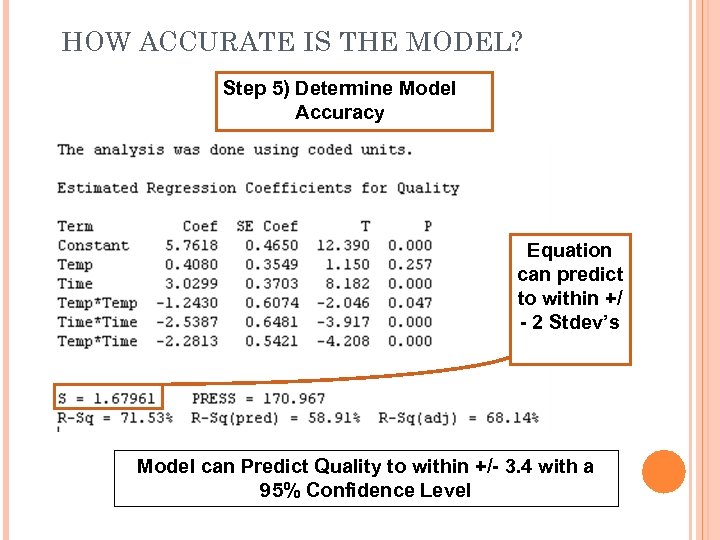
HOW ACCURATE IS THE MODEL? Step 5) Determine Model Accuracy Equation can predict to within +/ - 2 Stdev’s Model can Predict Quality to within +/- 3. 4 with a 95% Confidence Level

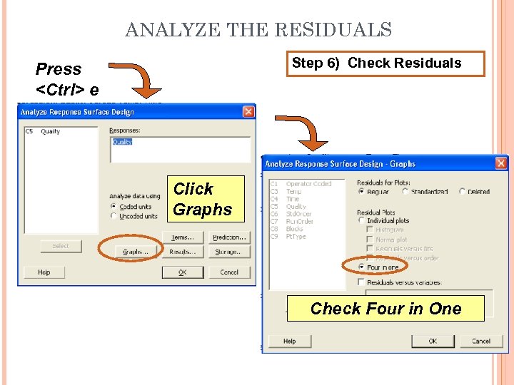
ANALYZE THE RESIDUALS Step 6) Check Residuals Press <Ctrl> e Click Graphs Check Four in One

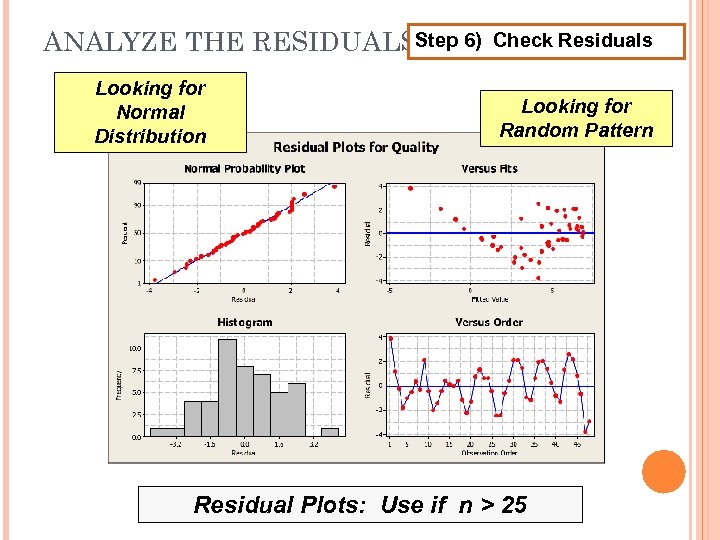
ANALYZE THE RESIDUALSStep 6) Looking for Normal Distribution Check Residuals Looking for Random Pattern Residual Plots: Use if n > 25

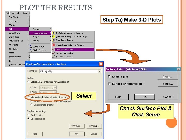
PLOT THE RESULTS Step 7 a) Make 3 -D Plots Select Check Surface Plot & Click Setup

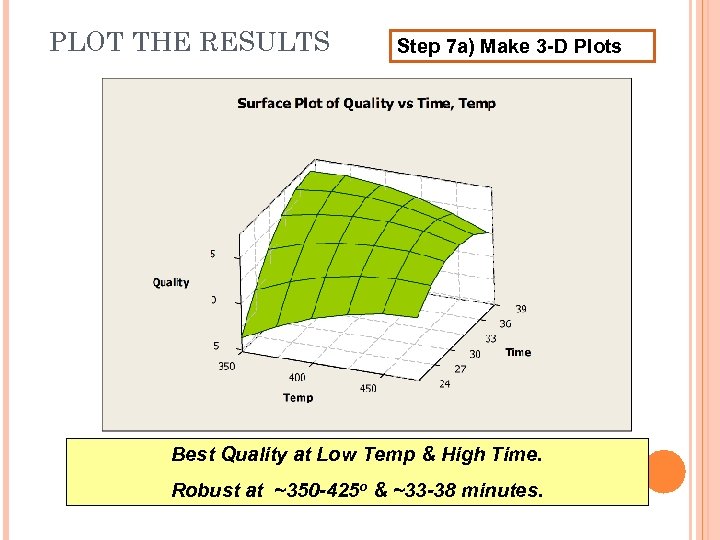
PLOT THE RESULTS Step 7 a) Make 3 -D Plots Best Quality at Low Temp & High Time. Robust at ~350 -425 o & ~33 -38 minutes.

EVALUATE THE RESULTS Step 8) Does the Results Make Sense EXPERIMENTAL RESULTS: • Numbers results matched up with original plotted data. • Operator didn’t matter to the results. • Lower oven temps & longer times result in the highest, most robust quality levels. • Are the results what you would have expected? • Are some statistically significant items not PRACTICALLY significant? • Looking at the 3 -D plot, do the changes in Temp & Time have a big enough effect on Quality to be useful?

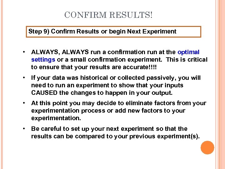
CONFIRM RESULTS! Step 9) Confirm Results or begin Next Experiment • ALWAYS, ALWAYS run a confirmation run at the optimal settings or a small confirmation experiment. This is critical to ensure that your results are accurate!!!! • If your data was historical or collected passively, you will need to run an experiment to show that your inputs CAUSED the changes to happen in your output. • At this point you may decide to eliminate factors from your experimentation process or add new factors to your experimentation. • Be careful to set up your next experiment so that the results can be compared to your previous experiment(s).

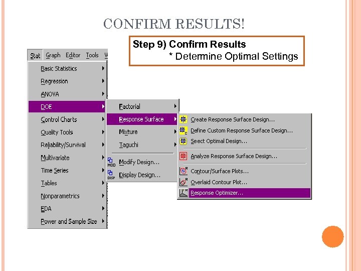
CONFIRM RESULTS! Step 9) Confirm Results * Determine Optimal Settings

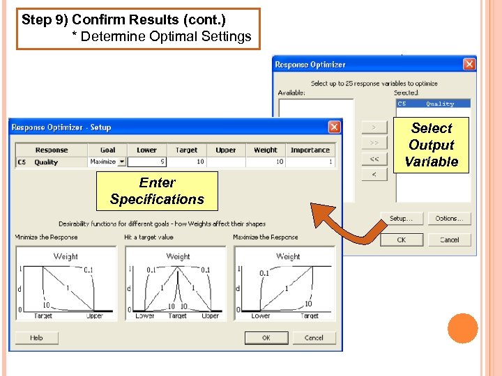
Step 9) Confirm Results (cont. ) * Determine Optimal Settings Select Output Variable Enter Specifications

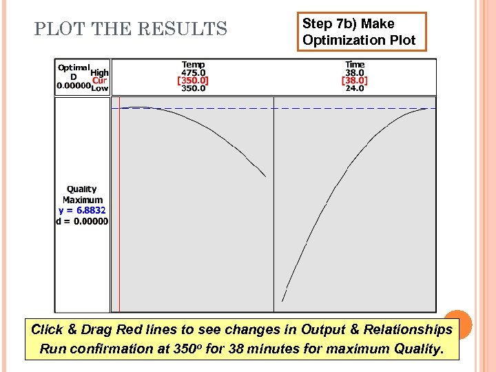
PLOT THE RESULTS Step 7 b) Make Optimization Plot Click & Drag Red lines to see changes in Output & Relationships Run confirmation at 350 o for 38 minutes for maximum Quality.

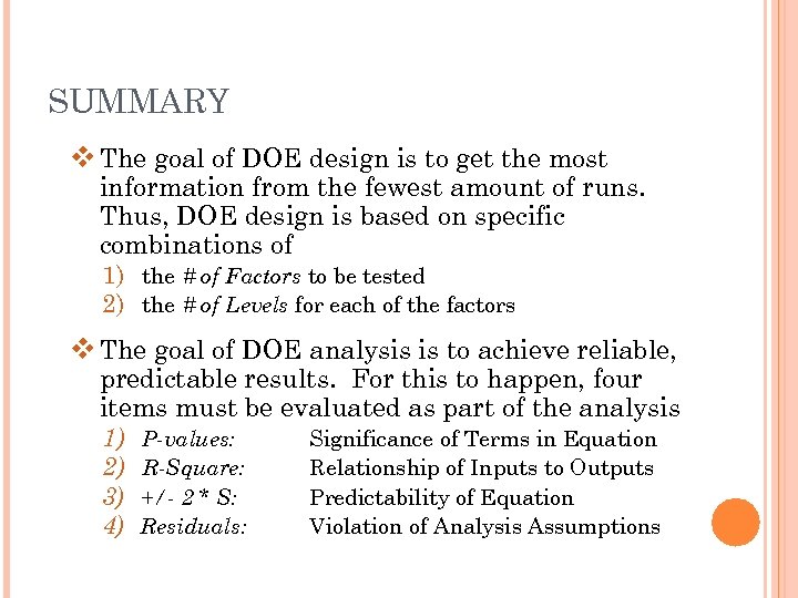
SUMMARY v The goal of DOE design is to get the most information from the fewest amount of runs. Thus, DOE design is based on specific combinations of 1) the # of Factors to be tested 2) the # of Levels for each of the factors v The goal of DOE analysis is to achieve reliable, predictable results. For this to happen, four items must be evaluated as part of the analysis 1) 2) 3) 4) P-values: R-Square: +/- 2 * S: Residuals: Significance of Terms in Equation Relationship of Inputs to Outputs Predictability of Equation Violation of Analysis Assumptions