DIurnal cycle Coupling Experiment DICE GLASS GASS

DIurnal cycle Coupling Experiment (DICE) GLASS / GASS joint project Martin Best and Adrian Lock © Crown copyright Met Office presented by Ayrton Zadra

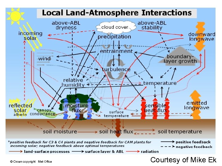© Crown copyright Met Office Courtesy of Mike Ek

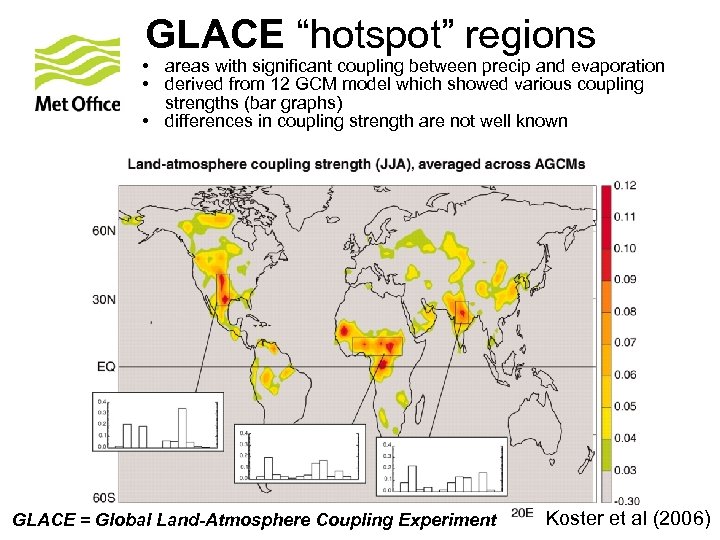GLACE “hotspot” regions • areas with significant coupling between precip and evaporation • derived from 12 GCM model which showed various coupling strengths (bar graphs) • differences in coupling strength are not well known GLACEcopyright Met Office © Crown = Global Land-Atmosphere Coupling Experiment Koster et al (2006)

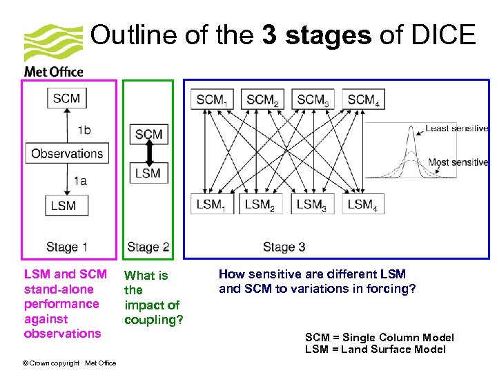Outline of the 3 stages of DICE LSM and SCM stand-alone performance against observations © Crown copyright Met Office What is the impact of coupling? How sensitive are different LSM and SCM to variations in forcing? SCM = Single Column Model LSM = Land Surface Model

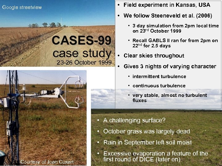• Field experiment in Kansas, USA Google streetview • We follow Steeneveld et al. (2006) CASES-99 case study 23 -26 October 1999 • 3 day simulation from 2 pm local time on 23 rd October 1999 • Recall GABLS II ran for from 2 pm on 22 nd for 2. 5 days • Clear skies throughout • Gives 3 nights of varying character • intermittent turbulence • continuous turbulence • very stable, almost no turbulent fluxes • A challenging surface? • October grass was largely dead • Rain in September left soil moist Courtesy of Joan Cuxart © Crown copyright Met Office • Excessive evaporation a feature of the first round of DICE (later on)

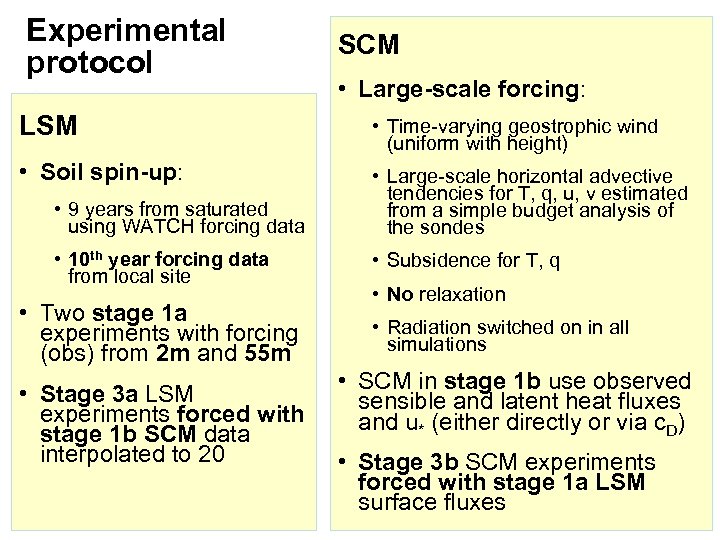Experimental protocol SCM • Large-scale forcing: LSM • Time-varying geostrophic wind (uniform with height) • Soil spin-up: • Large-scale horizontal advective tendencies for T, q, u, v estimated from a simple budget analysis of the sondes • 9 years from saturated using WATCH forcing data • 10 th year forcing data from local site • Two stage 1 a experiments with forcing (obs) from 2 m and 55 m • Stage 3 a LSM experiments forced with stage 1 b SCM data interpolated to 20 © Crown copyright Met Office • Subsidence for T, q • No relaxation • Radiation switched on in all simulations • SCM in stage 1 b use observed sensible and latent heat fluxes and u* (either directly or via c. D) • Stage 3 b SCM experiments forced with stage 1 a LSM surface fluxes

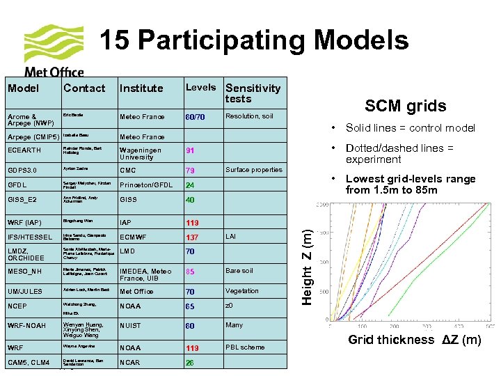15 Participating Models Model Contact Institute Levels Sensitivity Arome & Arpege (NWP) Eric Bazile Meteo France 60/70 Arpege (CMIP 5) Isabelle Beau Meteo France ECEARTH Reinder Ronda, Bert Holtslag Wageningen University 91 GDPS 3. 0 Ayrton Zadra CMC 79 GFDL Sergey Malyshev, Kirsten Findell Princeton/GFDL 24 GISS_E 2 Ann Fridlind, Andy Ackerman GISS 40 WRF (IAP) Bingcheng Wan IAP 119 IFS/HTESSEL Irina Sandu, Gianpaolo Balsamo ECMWF 137 LMDZ, ORCHIDEE Sonia Ait-Mesbah, Marie. Pierre Lefebvre, Frederique Cheruy LMD 70 MESO_NH Maria Jimenez, Patrick Le. Moigne, Joan Cuxart IMEDEA, Meteo France, UIB 85 Bare soil UM/JULES Adrian Lock, Martin Best Met Office 70 Vegetation NCEP Weizhong Zheng, NOAA 65 z 0 tests SCM grids Resolution, soil • Solid lines = control model • Dotted/dashed lines = experiment Surface properties Height Z (m) LAI • Lowest grid-levels range from 1. 5 m to 85 m Mike Ek WRF-NOAH Wenyan Huang, Xinyong Shen, Weiguo Wang NUIST 60 Many WRF Wayne Angevine NOAA 119 PBL scheme David Lawrence, Ben CAM 5, CLM 4 NCAR Sanderson © Crown copyright Met Office 26 Grid thickness ΔZ (m)

Highlights from stages 1 and 2 © Crown copyright Met Office

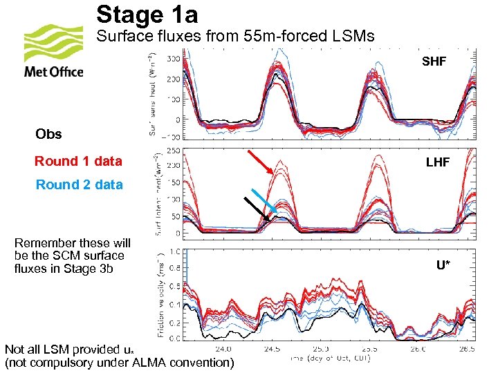Stage 1 a Surface fluxes from 55 m-forced LSMs SHF Obs Round 1 data LHF Round 2 data Remember these will be the SCM surface fluxes in Stage 3 b Not all LSM provided u* © compulsory Office (not Crown copyright Metunder ALMA convention) U*

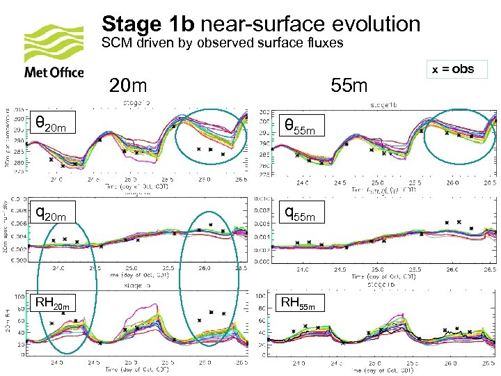Stage 1 b near-surface evolution SCM driven by observed surface fluxes 20 m 55 m θ 20 m θ 55 m q 20 m q 55 m RH 20 m RH 55 m © Crown copyright Met Office x = obs

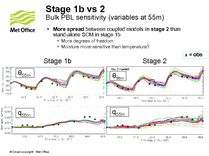Stage 1 b vs 2 Bulk PBL sensitivity (variables at 55 m) • More spread between coupled models in stage 2 than stand-alone SCM in stage 1 b • More degrees of freedom • Moisture more sensitive than temperature? Stage 2 Stage 1 b θ 55 m q 55 m © Crown copyright Met Office x = obs

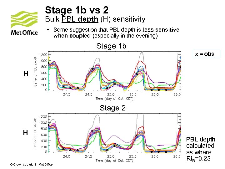Stage 1 b vs 2 Bulk PBL depth (H) sensitivity • Some suggestion that PBL depth is less sensitive when coupled (especially in the evening) Stage 1 b x = obs H Stage 2 H © Crown copyright Met Office PBL depth calculated as where Ri. B=0. 25

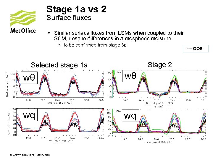Stage 1 a vs 2 Surface fluxes • Similar surface fluxes from LSMs when coupled to their SCM, despite differences in atmospheric moisture • to be confirmed from stage 3 a Stage 2 Selected stage 1 a wθ wθ wq wq © Crown copyright Met Office --- obs

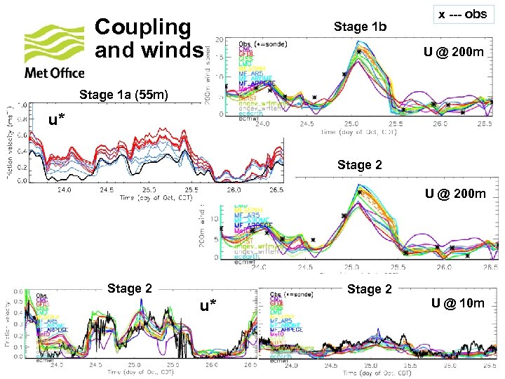Coupling and winds Stage 1 b x --- obs U @ 200 m Stage 1 a (55 m) u* Stage 2 U @ 200 m Stage 2 u* © Crown copyright Met Office Stage 2 U @ 10 m

Stage 3 a Surface flux sensitivities © Crown copyright Met Office

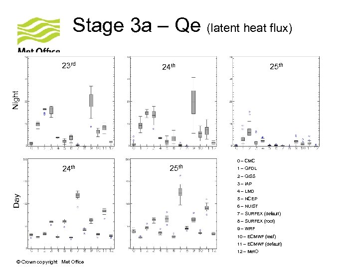Stage 3 a – Qe (latent heat flux) 25 th 24 th Night 23 rd 24 th 25 th 0 – CMC 1 – GFDL 2 – GISS 3 – IAP Day 4 – LMD 5 – NCEP 6 – NUIST 7 – SURFEX (default) 8 – SURFEX (root) 9 – WRF 10 – ECMWF (leaf) 11 – ECMWF (default) 12 – Met. O © Crown copyright Met Office

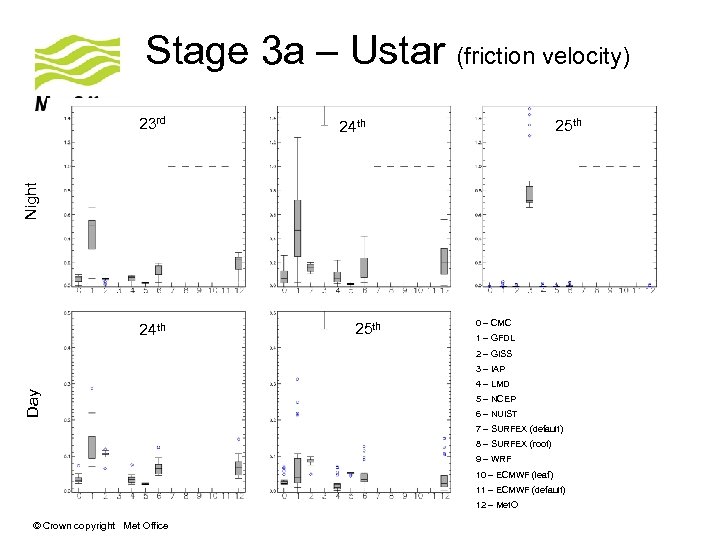Stage 3 a – Ustar (friction velocity) 25 th 24 th Night 23 rd 24 th 25 th 0 – CMC 1 – GFDL 2 – GISS 3 – IAP Day 4 – LMD 5 – NCEP 6 – NUIST 7 – SURFEX (default) 8 – SURFEX (root) 9 – WRF 10 – ECMWF (leaf) 11 – ECMWF (default) 12 – Met. O © Crown copyright Met Office

Stage 3 b Daytime sensitivities © Crown copyright Met Office

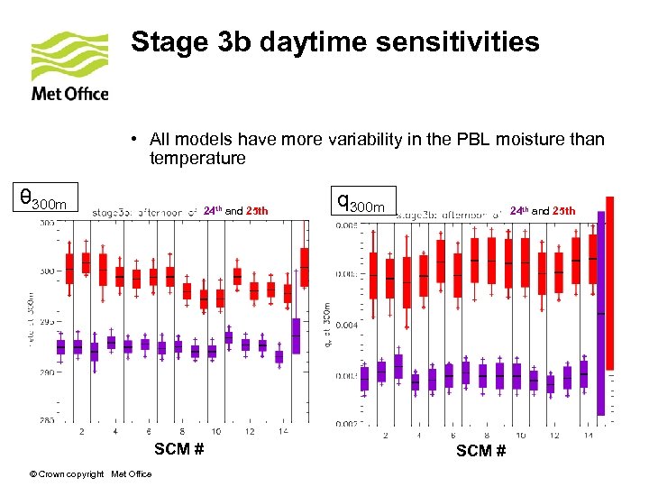Stage 3 b daytime sensitivities • All models have more variability in the PBL moisture than temperature θ 300 m 24 th and 25 th SCM # © Crown copyright Met Office q 300 m 24 th and 25 th SCM #

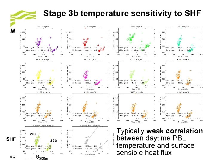Stage 3 b temperature sensitivity to SHF 24 th SHF 25 th θ 300 m © Crown copyright Met Office Typically weak correlation between daytime PBL temperature and surface sensible heat flux

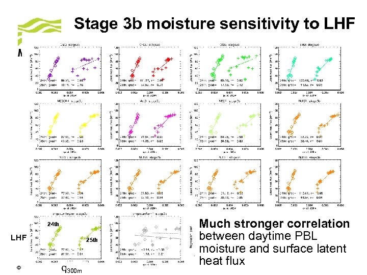Stage 3 b moisture sensitivity to LHF 24 th LHF 25 th q 300 m © Crown copyright Met Office Much stronger correlation between daytime PBL moisture and surface latent heat flux

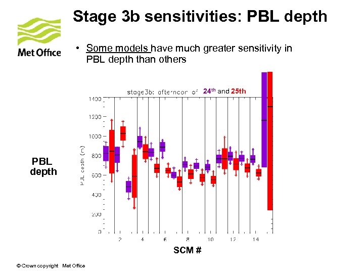Stage 3 b sensitivities: PBL depth • Some models have much greater sensitivity in PBL depth than others 24 th and 25 th PBL depth SCM # © Crown copyright Met Office

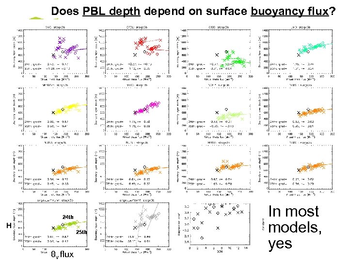Does PBL depth depend on surface buoyancy flux? 24 th H 25 th θv flux © Crown copyright Met Office In most models, yes

Stage 3 b Nighttime sensitivities © Crown copyright Met Office

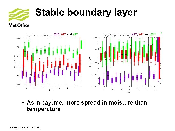Stable boundary layer 23 rd, 24 th and 25 th • As in daytime, more spread in moisture than temperature © Crown copyright Met Office

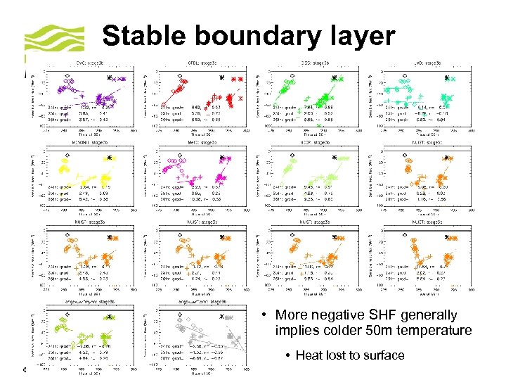
Stable boundary layer • More negative SHF generally implies colder 50 m temperature • Heat lost to surface © Crown copyright Met Office

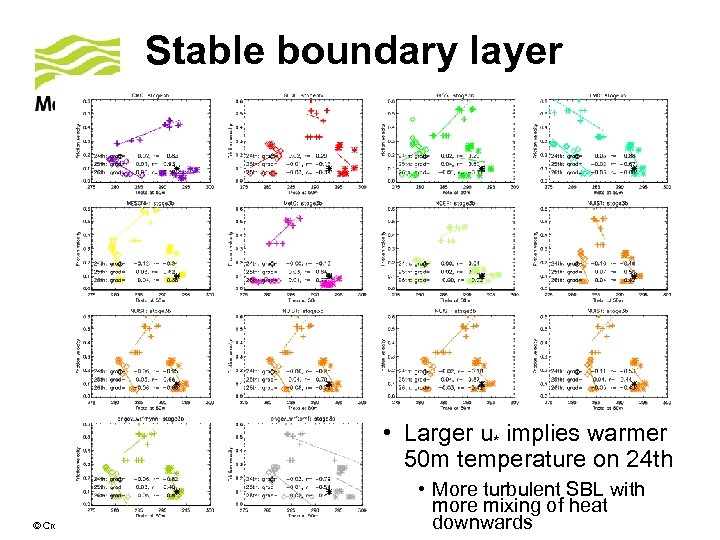
Stable boundary layer • Larger u* implies warmer 50 m temperature on 24 th © Crown copyright Met Office • More turbulent SBL with more mixing of heat downwards

DICE: summary so far More details at http: //appconv. metoffice. com/dice. html • Simple case (clear skies, no precipitation, homogeneous surface) but still a challenge for models • Climatalogical vegetation in LSMs can lead to large errors in evaporation • This dominated any signal of the impact of coupling in first round • Second round those LSMs that needed to constrained evaporation (adjusting LAI, root depth, bare soil behaviour) • Further discussion/developments are required to establish the best way to improve models • Early results indicate interesting differences in different models’ sensitivity to changes in forcing that are likely to be important in GCMs and need to be understood • Recent DICE discussions took place at the GEWEX conference, July 2014: • Planned reruns: additional data from stage 1 a, revised stage 3 b forcing data • Papers: • Martin Best and Adrian Lock to write up intercomparison (overview paper plus two separate papers on LSM and SCM analyses, respectively) • Special issue (eg BLM): to include participants' own analyses, model sensitivities, etc © Crown copyright Met Office

Merci ! © Crown copyright Met Office

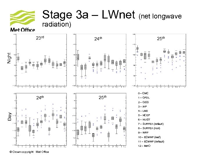Stage 3 a – LWnet (net longwave radiation) 25 th 24 th Night 23 rd 24 th 25 th 0 – CMC 1 – GFDL 2 – GISS 3 – IAP Day 4 – LMD 5 – NCEP 6 – NUIST 7 – SURFEX (default) 8 – SURFEX (root) 9 – WRF 10 – ECMWF (leaf) 11 – ECMWF (default) 12 – Met. O © Crown copyright Met Office

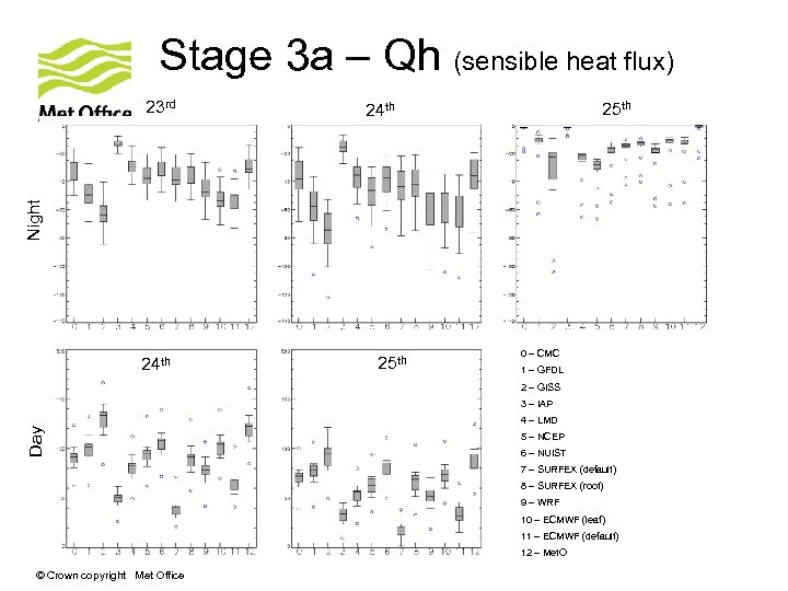Stage 3 a – Qh (sensible heat flux) 25 th 24 th Night 23 rd 24 th 25 th 0 – CMC 1 – GFDL 2 – GISS 3 – IAP Day 4 – LMD 5 – NCEP 6 – NUIST 7 – SURFEX (default) 8 – SURFEX (root) 9 – WRF 10 – ECMWF (leaf) 11 – ECMWF (default) 12 – Met. O © Crown copyright Met Office

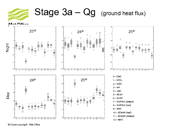Stage 3 a – Qg 25 th 24 th Night 23 rd (ground heat flux) 24 th 25 th 0 – CMC 1 – GFDL 2 – GISS 3 – IAP Day 4 – LMD 5 – NCEP 6 – NUIST 7 – SURFEX (default) 8 – SURFEX (root) 9 – WRF 10 – ECMWF (leaf) 11 – ECMWF (default) 12 – Met. O © Crown copyright Met Office

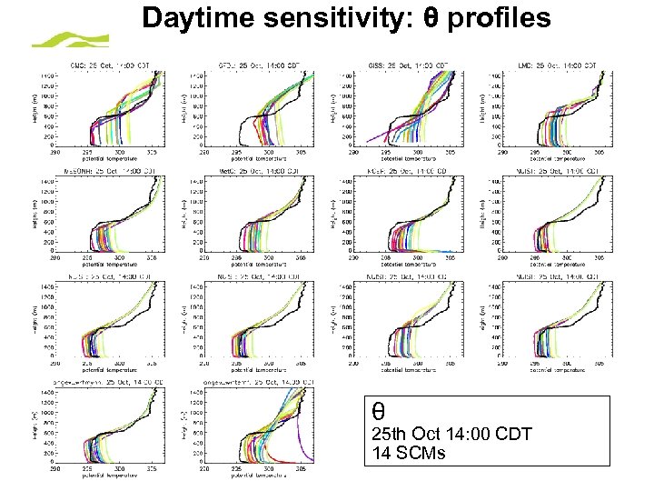Daytime sensitivity: θ profiles θ 25 th Oct 14: 00 CDT 14 SCMs © Crown copyright Met Office

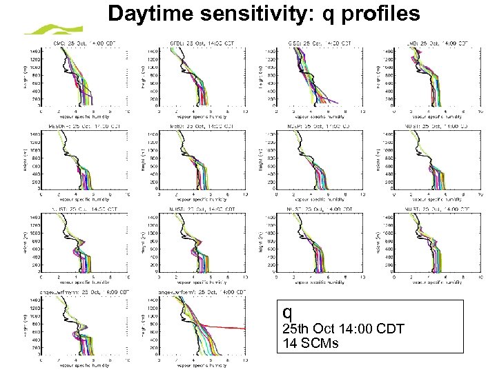Daytime sensitivity: q profiles q 25 th Oct 14: 00 CDT 14 SCMs © Crown copyright Met Office

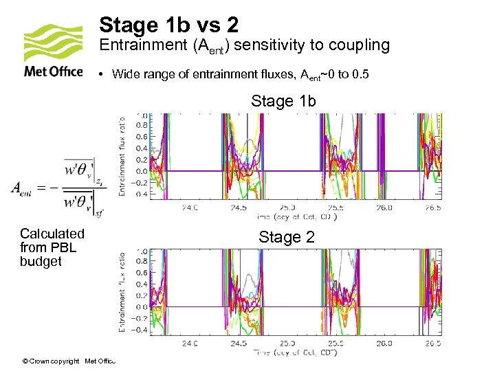
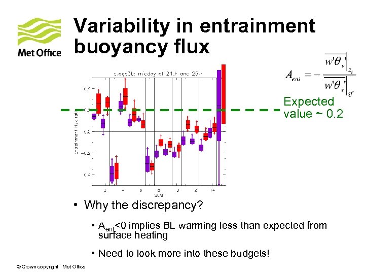Variability in entrainment buoyancy flux Expected value ~ 0. 2 • Why the discrepancy? • Aent<0 implies BL warming less than expected from surface heating • Need to look more into these budgets! © Crown copyright Met Office

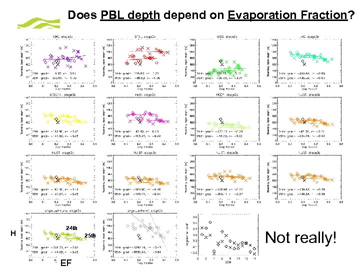Does PBL depth depend on Evaporation Fraction? H 24 th 25 th EF © Crown copyright Met Office Not really!

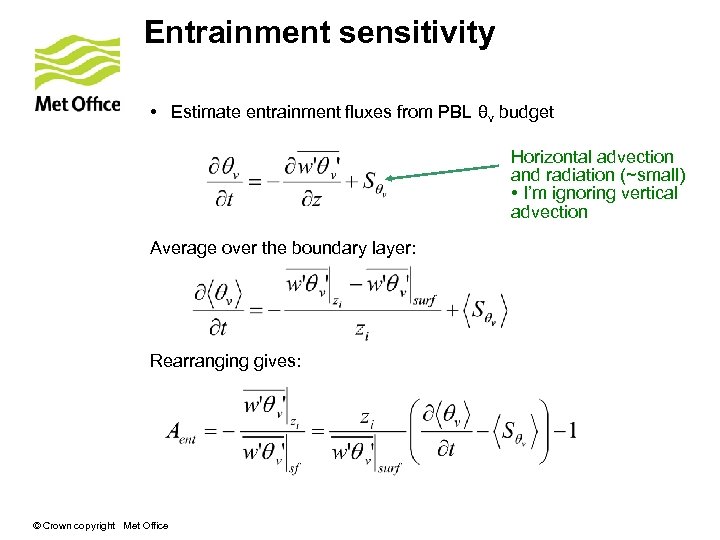Entrainment sensitivity • Estimate entrainment fluxes from PBL θv budget Horizontal advection and radiation (~small) • I’m ignoring vertical advection Average over the boundary layer: Rearranging gives: © Crown copyright Met Office

Stage 1 b vs 2 Entrainment (Aent) sensitivity to coupling • Wide range of entrainment fluxes, Aent~0 to 0. 5 Stage 1 b Calculated from PBL budget © Crown copyright Met Office Stage 2

Stable boundary layer • More negative SHF generally implies colder 50 m temperature • Heat lost to surface © Crown copyright Met Office

Stable boundary layer • Larger u* implies warmer 50 m temperature on 24 th © Crown copyright Met Office • More turbulent SBL with more mixing of heat downwards