Distributed Database Management Systems Lecture 33 In

Зарегистрируйтесь, чтобы просмотреть полный документ!

РЕГИСТРАЦИЯ

Distributed Database Management Systems Lecture 33

In the previous lecture • Final phase of QD • Data Localization: for HF, VF and DF.

In today’s Lecture • Data Localization for Hybrid Fragmentation • Query Optimization.

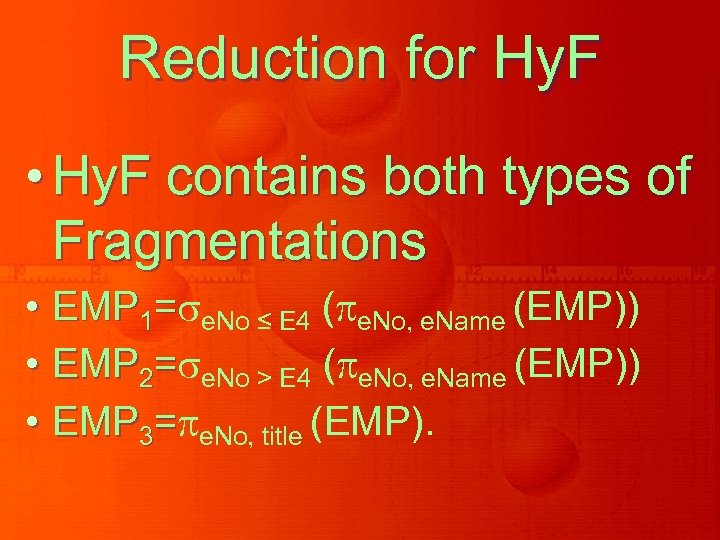
Reduction for Hy. F • Hy. F contains both types of Fragmentations • EMP 1= e. No ≤ E 4 ( e. No, e. Name (EMP)) • EMP 2= e. No > E 4 ( e. No, e. Name (EMP)) • EMP 3= e. No, title (EMP).

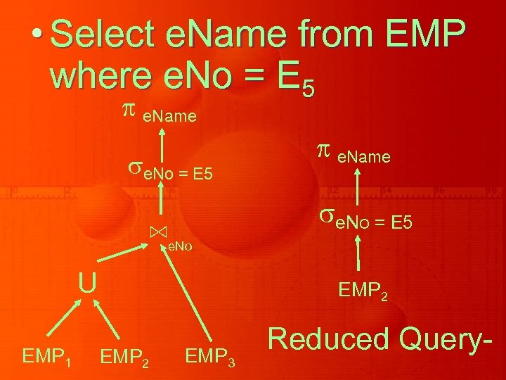
• Select e. Name from EMP where e. No = E 5 e. Name e. No = E 5 ⋈ e. No U EMP 1 EMP 2 EMP 3 Reduced Query-

Summary of what we have done so far

• Query Decomposition: generates an efficient query in relational algebra – Normalization, Analysis, Simplification, Rewriting • Data Localization: applies global query to fragments; increases optimization level-

• So, next is the cost-based optimization • Mainly concentrates on the order of performing joins • Characteristics of relations like cardinalities are considered

• First QO in general • QO refers to producing a Query Execution plan (QEP) that represents execution strategy.

• Components of Optimizer • Search Space: set of eq. alternative exec plans • Cost Model: predicts cost of a execution plan • Search Strategy: produces best plan

Search Space • Search space consists of eq. Query Trees produced using Tr Rules • Optimizer concentrates on join trees, since join cost is the most effective

• Example: • Select e. Name, resp From EMP, ASG, PROJ where EMP. e. No = ASG. e. No and ASG. p. No = PROJ. p. No.

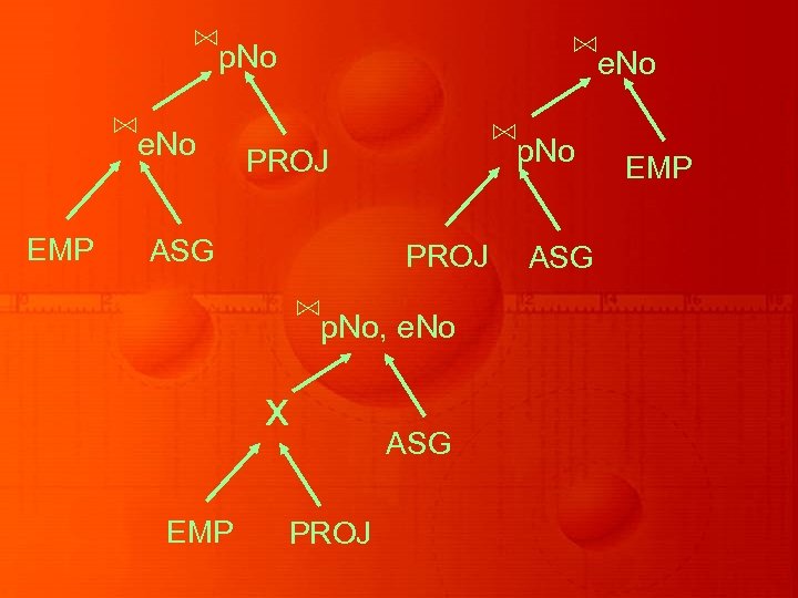
⋈p. No ⋈e. No EMP ⋈e. No ⋈p. No PROJ ASG PROJ ⋈p. No, e. No x EMP ASG PROJ ASG EMP

• Alternatives with N relations are O(N!) based on properties of relations • So, restrictions are applied

1 - Heuristics - Selection and projection on base relations - Avoid Cartesian product

2 - Shape of Tree - Linear Tree: At least one node for each operand is a base relation - Bushy tree: May have operators with interm tables only; allows parallel execution

Search Strategy • Most popular is Dynamic Programming • That starts with base relations and keeps on adding relations calculating cost

• DP is almost exhaustive so produces best plan • Too expensive with more than 5 relations • Other option is Randomized strategy • Do not guarantee best

Cost Model • Cost of operators, statistics of base data to predict size of intermediate tables • Cost considered as Total Time and Response Time.

• Total time = CPU time + I/O time + tr time • In WAN, major cost is tr time • Initially ratios were 20: 1 for tr and I/O, for LAN it is 1: 1. 6

• Response time = CPU time + I/O time + tr time • Difference. ?

• TCPU = time for a CPU inst • TI/O = a disk I/O • TMSG = fixed time for initiating and recv a msg • TTR = transmit a data unit from one site to another.

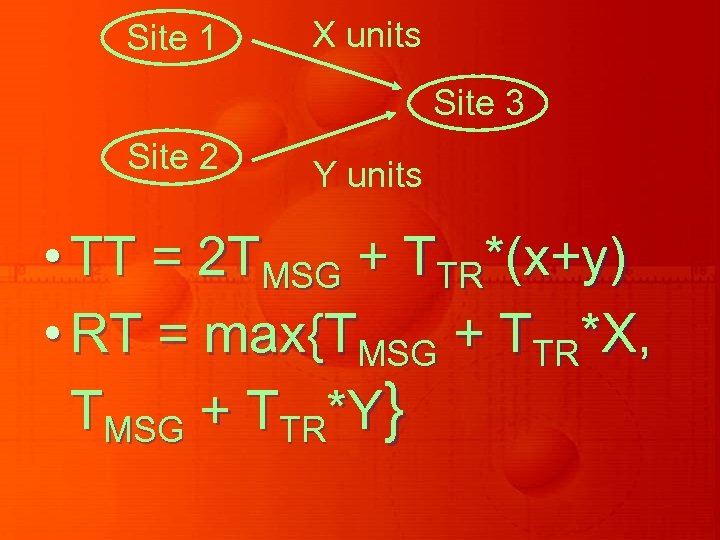
Site 1 X units Site 3 Site 2 Y units • TT = 2 TMSG + TTR*(x+y) • RT = max{TMSG + TTR*X, TMSG + TTR*Y}

Database Statistics • Major factor is interm tabs • If the interm results are to be transmitted, then estimation about size is a must • More precise statistics cost more

• For each relation R[A 1, A 2, …, An] fragmented as R 1, …, Rr 1. length of each attribute: length(Ai) 2. the number of distinct values for each attribute in each fragment: card( Ai(Rj)) 3. maximum and minimum values in the domain of each attribute: min(Ai), max(Ai).

4. The cardinalities of each domain: card(dom[Ai]) and the cardinalities of each fragment: card(Rj) 5. Join selectivity factor for some of the relations SFJ (R, S) = card(R ⋈ S)/ (card(R) ∗ card(S))-

Cardinalities of Intermediate Results

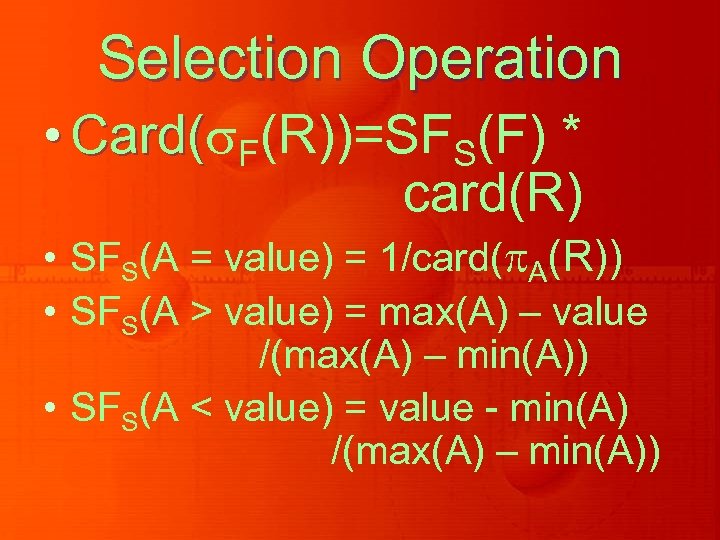
Selection Operation • Card( F(R))=SFS(F) * Card( card(R) • SFS(A = value) = 1/card( A(R)) • SFS(A > value) = max(A) – value /(max(A) – min(A)) • SFS(A < value) = value - min(A) /(max(A) – min(A))

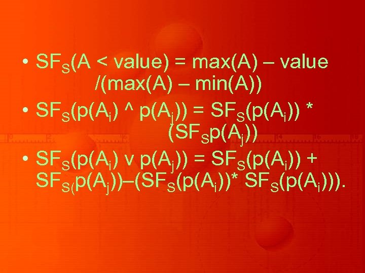
• SFS(A < value) = max(A) – value /(max(A) – min(A)) • SFS(p(Ai) ^ p(Aj)) = SFS(p(Ai)) * (SFSp(Aj)) • SFS(p(Ai) v p(Aj)) = SFS(p(Ai)) + SFS(p(Aj))–(SFS(p(Ai))* SFS(p(Ai))).

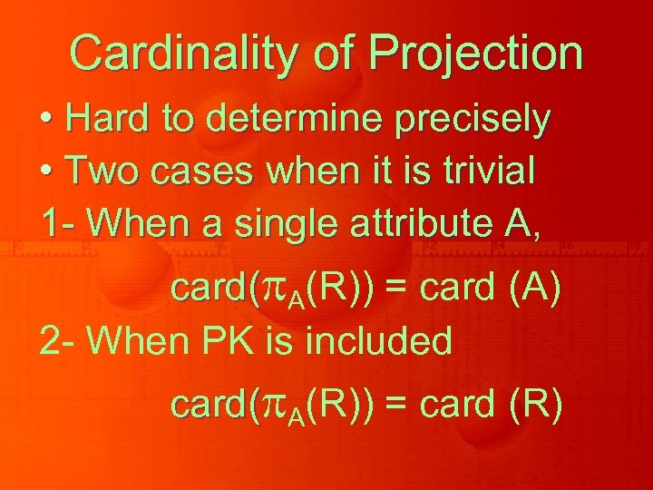
Cardinality of Projection • Hard to determine precisely • Two cases when it is trivial 1 - When a single attribute A, card( A(R)) = card (A) 2 - When PK is included card( A(R)) = card (R)

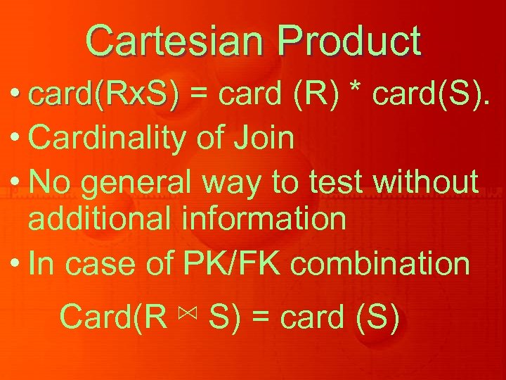
Cartesian Product • card(Rx. S) = card (R) * card(S). • Cardinality of Join • No general way to test without additional information • In case of PK/FK combination Card(R ⋈ S) = card (S)

• Semi Join: SFSJ(R ⋉AS)= card( A(S))/ card(dom[A]) card(R ⋉AS) = SFSJ(S. A) * card(R).

• Union: Hard to estimate • Limits possible which are card(R) + card(S) and max{card (R) + card (S)) • Difference: Like Union, card (R) for (R-S), and 0

Centralized Query Optimization

Why to Study 1. Distributed Query is transformed into local ones 2. Issues are related and more complex in DD 3. Easier to understand • Two famous ones.

• INGRES – Dynamic – Recursively breaks into smaller ones • System R –static –exhaustive search

Скачать презентацию Distributed Database Management Systems Lecture 33 In

399445c6b839c32f6f79e6615965a6ca.ppt

Количество слайдов: 36