Discrete Maths 241 -303 Semester 1 2014 -2015

Discrete Maths 241 -303, Semester 1 2014 -2015 6. Trees • Objective – introduce more unusual tree algorithms and techniques • you already know about binary (search) trees 241 -303 Discrete Maths: Trees/6 1

Overview. 1. 2 ). 3 Uses of Trees Huffman Codes Rooted) Tree Terminology . 4 Spanning Trees . 5 Minimal Spanning Trees . 6. 7 Game Trees More Information 241 -303 Discrete Maths: Trees/6 2

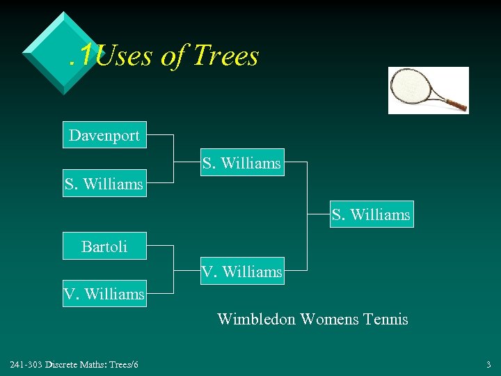. 1 Uses of Trees Davenport S. Williams Bartoli V. Williams Wimbledon Womens Tennis 241 -303 Discrete Maths: Trees/6 3

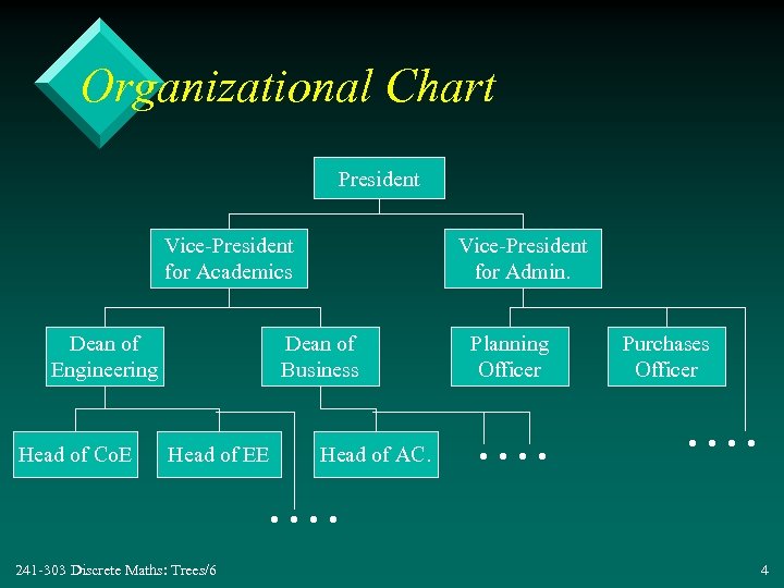Organizational Chart President Vice-President for Academics Dean of Engineering Head of Co. E Vice-President for Admin. Dean of Business Head of EE Head of AC. Planning Officer . . Purchases Officer . . . . 241 -303 Discrete Maths: Trees/6 4

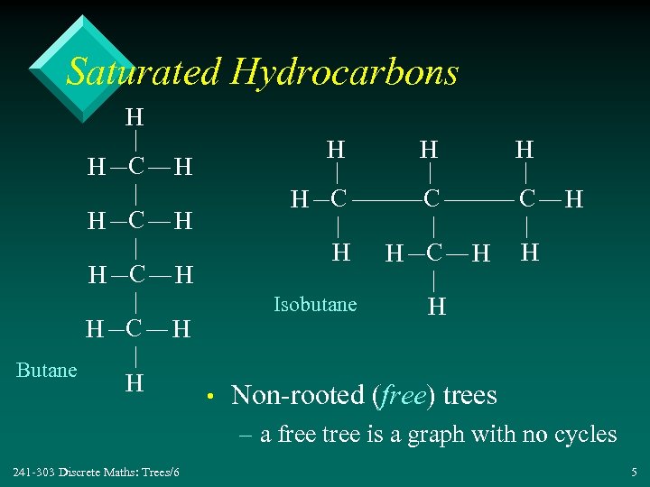Saturated Hydrocarbons H H C H C Butane H H C Isobutane H H C H H • H H Non-rooted (free) trees – a free tree is a graph with no cycles 241 -303 Discrete Maths: Trees/6 5

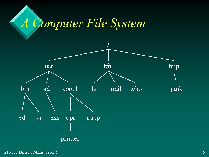A Computer File System / usr bin ed ad vi bin spool exs opr ls mail tmp who junk uucp printer 241 -303 Discrete Maths: Trees/6 6

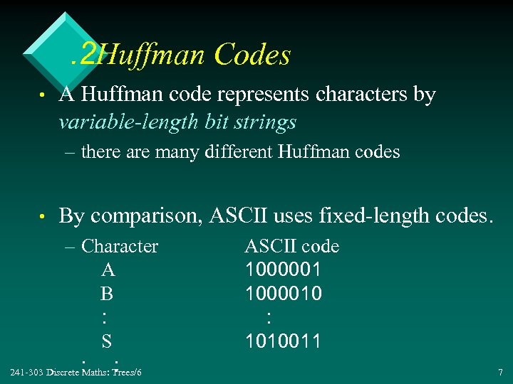. 2 Huffman Codes • A Huffman code represents characters by variable-length bit strings – there are many different Huffman codes • By comparison, ASCII uses fixed-length codes. – Character A B : S : 241 -303 Discrete : Maths: Trees/6 ASCII code 1000001 1000010 : 1010011 7

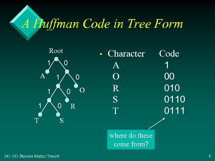A Huffman Code in Tree Form Root 1 A • 0 1 1 1 0 0 0 T R O Character A O R S T Code 1 00 0110 0111 S where do these come from? 241 -303 Discrete Maths: Trees/6 8

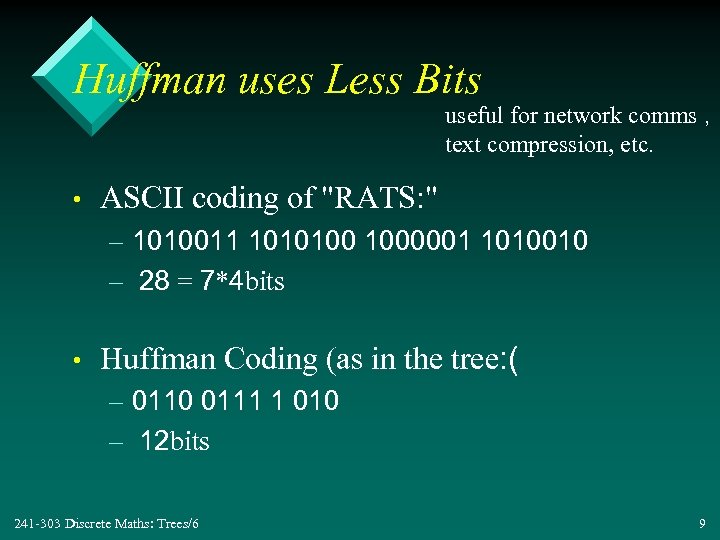Huffman uses Less Bits useful for network comms , text compression, etc. • ASCII coding of "RATS: " – 1010011 1010100 1000001 1010010 – 28 = 7*4 bits • Huffman Coding (as in the tree: ( – 0110 0111 1 010 – 12 bits 241 -303 Discrete Maths: Trees/6 9

Constructing a Huffman Code • A Huffman code is based on a table giving the frequency of the characters in the 'language. ' • The 'language' can be a subset of a full language – e. g. business English, computer language keywords, the months of the year, a language made up of only {A, O, R, S, T{ 241 -303 Discrete Maths: Trees/6 10

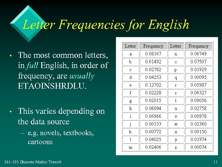Letter Frequencies for English • The most common letters, in full English, in order of frequency, are usually ETAOINSHRDLU. • This varies depending on the data source – e. g. novels, textbooks, cartoons 241 -303 Discrete Maths: Trees/6 11

Example: The Haddock Language • The Haddock language contains only 5 characters: – % , $ , # , @ , ! – we can make words like: • • @@@@@#$%$@@!!! We must create a frequency table by analysing existing examples of Haddock writing. 241 -303 Discrete Maths: Trees/6 continued 12

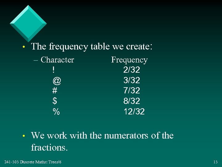• The frequency table we create: – Character ! @ # $ % • Frequency 2/32 3/32 7/32 8/32 12/32 We work with the numerators of the fractions. 241 -303 Discrete Maths: Trees/6 13

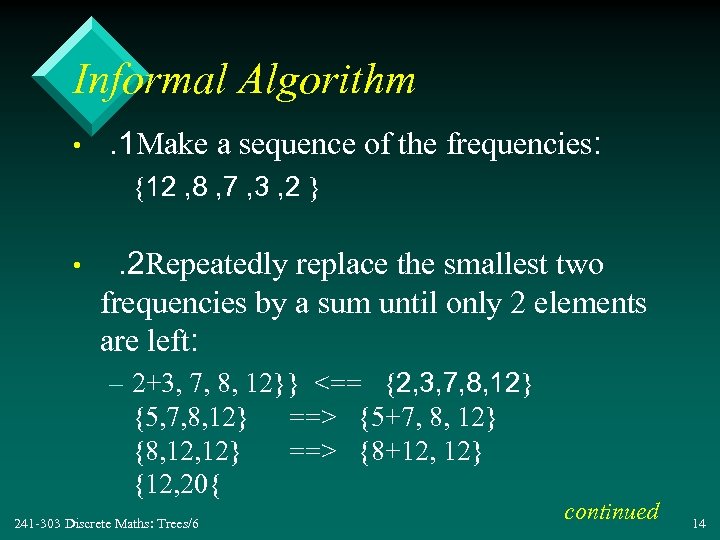Informal Algorithm • . 1 Make a sequence of the frequencies: {12 , 8 , 7 , 3 , 2 } • . 2 Repeatedly replace the smallest two frequencies by a sum until only 2 elements are left: – 2+3, 7, 8, 12}} <== {2, 3, 7, 8, 12} {5, 7, 8, 12} ==> {5+7, 8, 12} {8, 12} ==> {8+12, 12} {12, 20{ 241 -303 Discrete Maths: Trees/6 continued 14

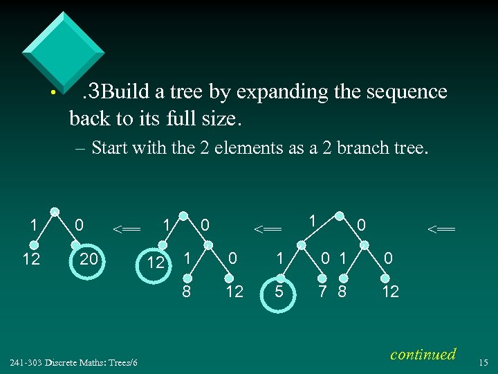• . 3 Build a tree by expanding the sequence back to its full size. – Start with the 2 elements as a 2 branch tree. 1 0 <== 20 241 -303 Discrete Maths: Trees/6 12 1 0 1 0 8 12 12 5 7 8 12 continued 15

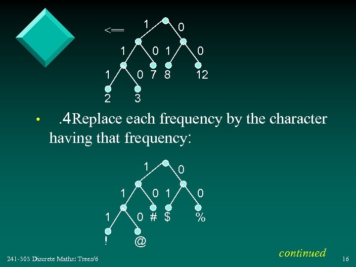1 <== 1 0 0 1 1 • 0 7 8 2 0 12 3 . 4 Replace each frequency by the character having that frequency: 1 1 0 0 1 0 # $ % ! 241 -303 Discrete Maths: Trees/6 0 1 @ continued 16

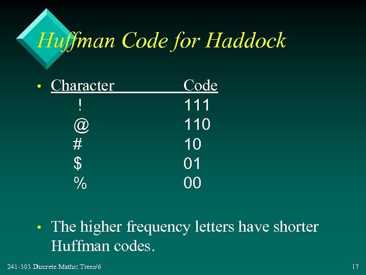Huffman Code for Haddock • Character ! @ # $ % • The higher frequency letters have shorter Huffman codes. 241 -303 Discrete Maths: Trees/6 Code 111 110 10 01 00 17

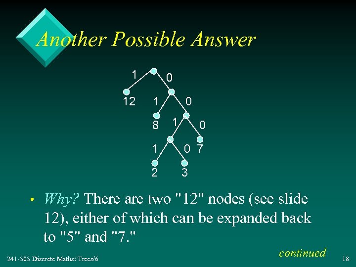Another Possible Answer 1 12 0 1 8 0 1 2 • 0 7 3 Why? There are two "12" nodes (see slide 12), either of which can be expanded back to "5" and "7. " 241 -303 Discrete Maths: Trees/6 continued 18

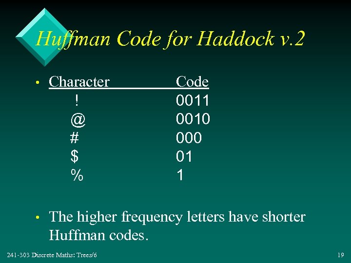Huffman Code for Haddock v. 2 • Character ! @ # $ % • The higher frequency letters have shorter Huffman codes. 241 -303 Discrete Maths: Trees/6 Code 0011 0010 000 01 1 19

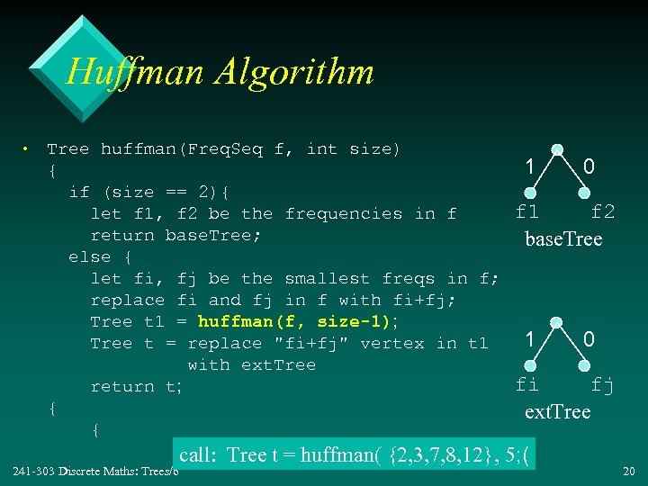Huffman Algorithm • Tree huffman(Freq. Seq f, int size) { if (size == 2){ let f 1, f 2 be the frequencies in f return base. Tree; else { let fi, fj be the smallest freqs in f; replace fi and fj in f with fi+fj; Tree t 1 = huffman(f, size-1); Tree t = replace "fi+fj" vertex in t 1 with ext. Tree return t; { { 241 -303 Discrete Maths: Trees/6 1 0 f 1 f 2 base. Tree 1 0 fi fj ext. Tree call: Tree t = huffman( {2, 3, 7, 8, 12}, 5; ( 20

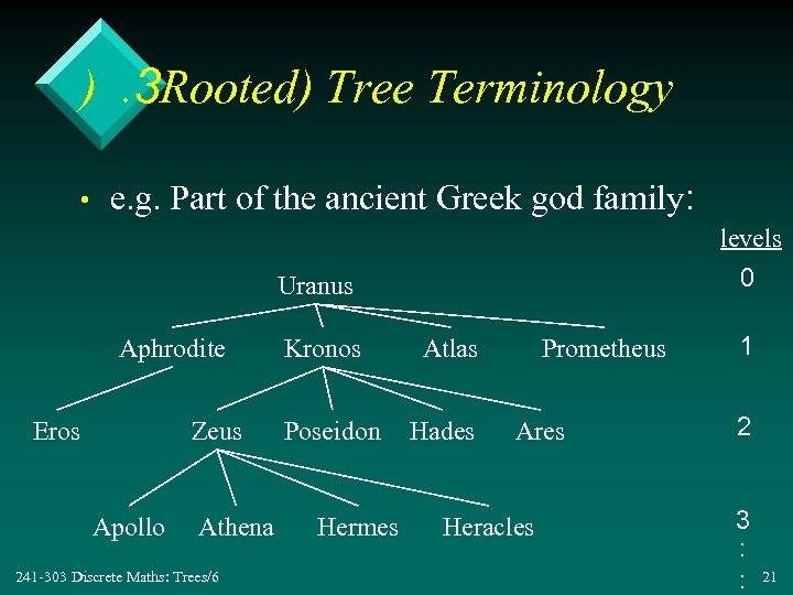). 3 Rooted) Tree Terminology • e. g. Part of the ancient Greek god family: levels 0 Uranus Aphrodite Eros Zeus Apollo Athena 241 -303 Discrete Maths: Trees/6 Kronos Poseidon Hermes Atlas Hades Prometheus Ares Heracles 1 2 3 : : 21

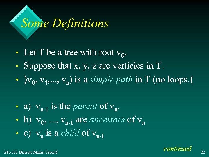Some Definitions • • • Let T be a tree with root v 0. Suppose that x, y, z are verticies in T. )v 0, v 1, . . . , vn) is a simple path in T (no loops. ( a) vn-1 is the parent of vn. b) v 0, . . . , vn-1 are ancestors of vn c) vn is a child of vn-1 241 -303 Discrete Maths: Trees/6 continued 22

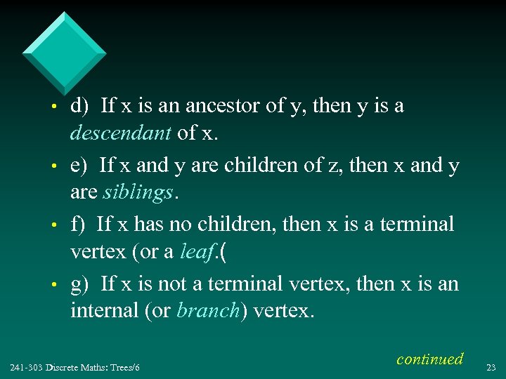• • d) If x is an ancestor of y, then y is a descendant of x. e) If x and y are children of z, then x and y are siblings. f) If x has no children, then x is a terminal vertex (or a leaf. ( g) If x is not a terminal vertex, then x is an internal (or branch) vertex. 241 -303 Discrete Maths: Trees/6 continued 23

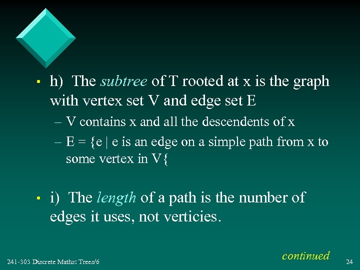• h) The subtree of T rooted at x is the graph with vertex set V and edge set E – V contains x and all the descendents of x – E = {e | e is an edge on a simple path from x to some vertex in V{ • i) The length of a path is the number of edges it uses, not verticies. 241 -303 Discrete Maths: Trees/6 continued 24

• j) The level of a vertex x is the length of the simple path from the root to x. • k) The height of a vertex x is the length of the simple path from x to the farthest leaf – the height of a tree is the height of its root • l) A tree where every internal vertex has exactly m children is called a full m-ary tree. 241 -303 Discrete Maths: Trees/6 25

Applied to the Example • • • The root is Uranus. A simple path is {Uranus, Aphrodite, Eros{ The parent of Eros is Aphrodite. The ancestors of Hermes are Zeus, Kronos, and Uranus. The children of Zeus are Apollo, Athena, Hermes, and Heracles. 241 -303 Discrete Maths: Trees/6 continued 26

• The descendants of Kronos are Zeus, Poseidon, Hades, Ares, Apollo, Athena, Hermes, and Heracles. • The leaves (terminal verticies) are Eros, Apollo, Athena, Hermes, Heracles, Poseidon, Hades, Ares, Atlas, and Prometheus. • The branches (internal verticies) are Uranus, Aphrodite, Kronos, and Zeus. 241 -303 Discrete Maths: Trees/6 continued 27

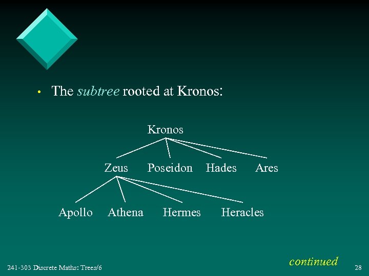• The subtree rooted at Kronos: Kronos Zeus Apollo 241 -303 Discrete Maths: Trees/6 Athena Poseidon Hermes Hades Ares Heracles continued 28

• The length of the path {Uranus, Aphrodite, Eros} is 2 (not 3. ( • The level of Ares is 2. • The height of the tree is 3. 241 -303 Discrete Maths: Trees/6 29

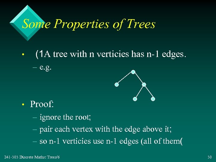Some Properties of Trees • (1 A tree with n verticies has n-1 edges. – e. g. • Proof: – ignore the root; – pair each vertex with the edge above it; – so n-1 verticies use n-1 edges (all of them( 241 -303 Discrete Maths: Trees/6 30

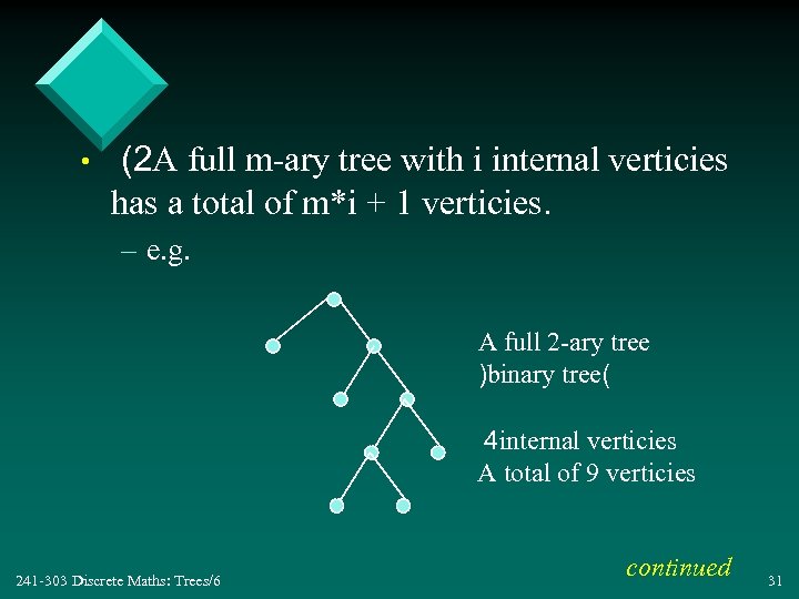• (2 A full m-ary tree with i internal verticies has a total of m*i + 1 verticies. – e. g. A full 2 -ary tree )binary tree( 4 internal verticies A total of 9 verticies 241 -303 Discrete Maths: Trees/6 continued 31

• Proof – ignore the root; – every remaining vertex is the child of an internal vertex; – each internal vertex has m children; – there are i internal verticies, so there is a total of m*i verticies in the tree; – add back the root, to get m*i + 1 241 -303 Discrete Maths: Trees/6 32

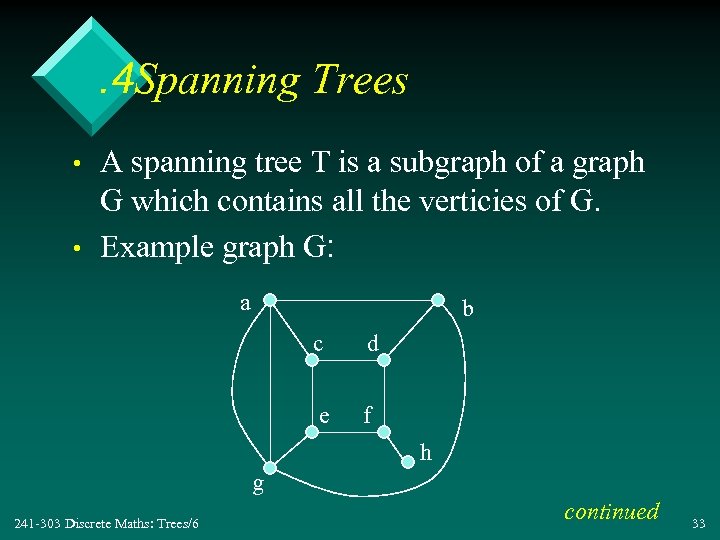. 4 Spanning Trees • • A spanning tree T is a subgraph of a graph G which contains all the verticies of G. Example graph G: a b c d e f h g 241 -303 Discrete Maths: Trees/6 continued 33

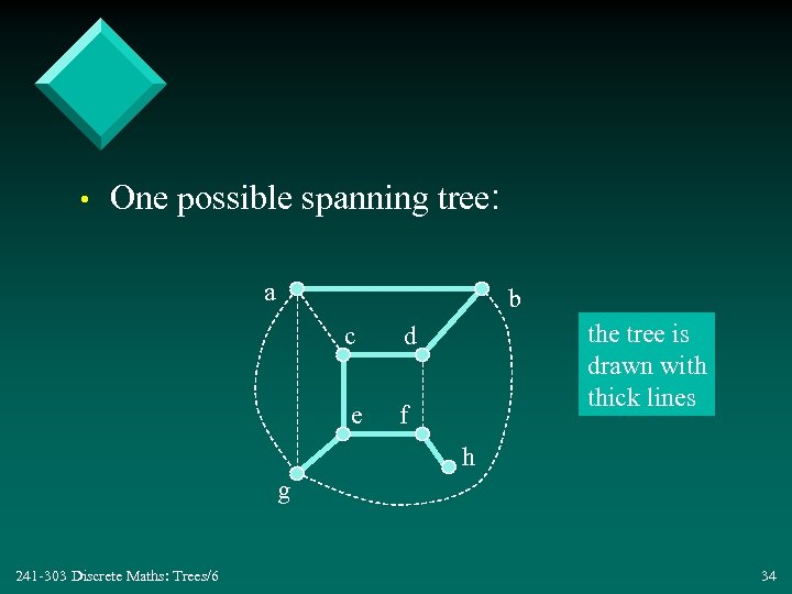• One possible spanning tree: a b c e the tree is drawn with thick lines d f h g 241 -303 Discrete Maths: Trees/6 34

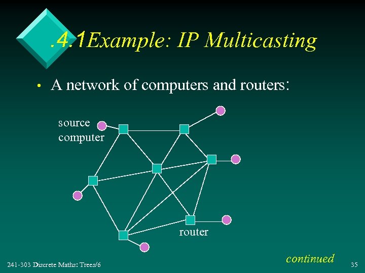. 4. 1 Example: IP Multicasting • A network of computers and routers: source computer router 241 -303 Discrete Maths: Trees/6 continued 35

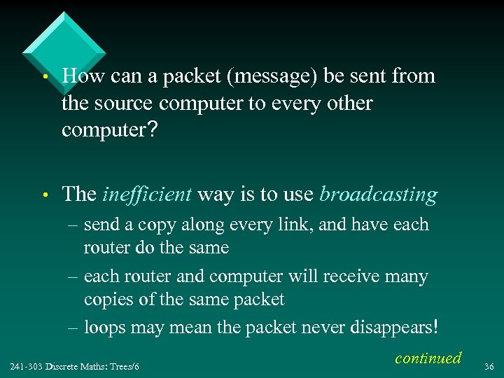• How can a packet (message) be sent from the source computer to every other computer? • The inefficient way is to use broadcasting – send a copy along every link, and have each router do the same – each router and computer will receive many copies of the same packet – loops may mean the packet never disappears! 241 -303 Discrete Maths: Trees/6 continued 36

• IP multicasting is an efficient solution – send a single packet to one router – have the router send it to 1 or more routers in such a way that a computer never receives the packet more than once • This behaviour can be represented by a spanning tree. 241 -303 Discrete Maths: Trees/6 continued 37

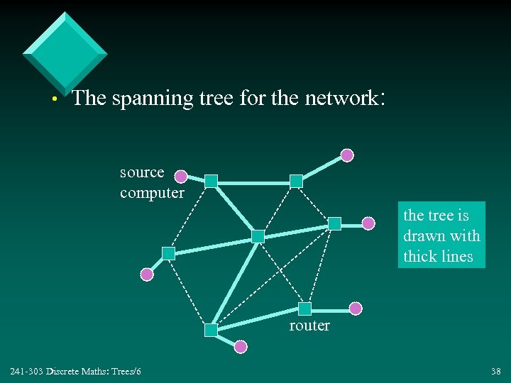• The spanning tree for the network: source computer the tree is drawn with thick lines router 241 -303 Discrete Maths: Trees/6 38

. 4. 2 Finding a Spanning Tree • There are two main types of algorithms: – breadth-first search – depth-first search 241 -303 Discrete Maths: Trees/6 39

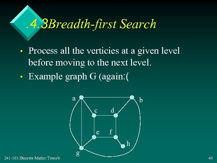. 4. 3 Breadth-first Search • • Process all the verticies at a given level before moving to the next level. Example graph G (again: ( a b c d e f h 241 -303 Discrete Maths: Trees/6 g 40

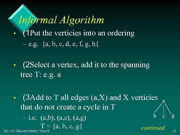Informal Algorithm • (1 Put the verticies into an ordering – e. g. {a, b, c, d, e, f, g, h{ • (2 Select a vertex, add it to the spanning tree T: e. g. a • (3 Add to T all edges (a, X) and X verticies that do not create a cycle in T a b c – i. e. (a, b), (a, c), (a, g) T = {a, b, c, g{ 241 -303 Discrete Maths: Trees/6 continued g 41

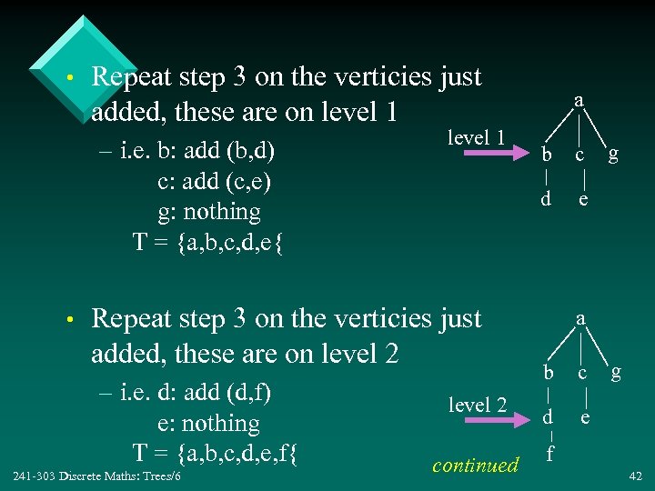• Repeat step 3 on the verticies just added, these are on level 1 – i. e. b: add (b, d) c: add (c, e) g: nothing T = {a, b, c, d, e{ • level 1 241 -303 Discrete Maths: Trees/6 level 2 continued b c d Repeat step 3 on the verticies just added, these are on level 2 – i. e. d: add (d, f) e: nothing T = {a, b, c, d, e, f{ a g e a b c d g e f 42

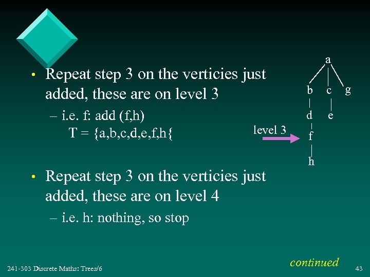• Repeat step 3 on the verticies just added, these are on level 3 – i. e. f: add (f, h) T = {a, b, c, d, e, f, h{ • a Repeat step 3 on the verticies just added, these are on level 4 c d level 3 b g e f h – i. e. h: nothing, so stop 241 -303 Discrete Maths: Trees/6 continued 43

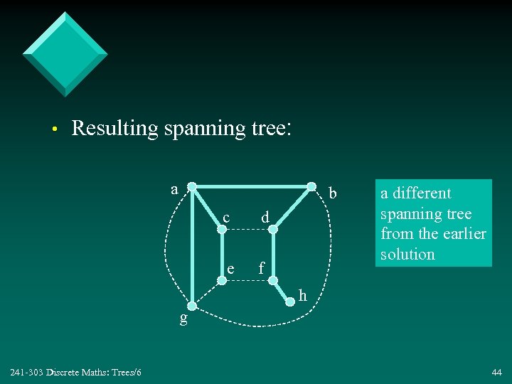• Resulting spanning tree: a b c d e f a different spanning tree from the earlier solution h g 241 -303 Discrete Maths: Trees/6 44

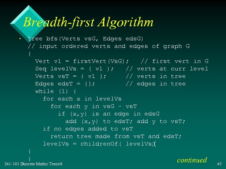Breadth-first Algorithm • Tree bfs(Verts vs. G, Edges eds. G) // input ordered verts and edges of graph G { Vert v 1 = first. Vert(Vs. G); // first vert in G Seq level. Vs = ( v 1 ); // verts at curr level Verts vs. T = { v 1 }; // verts in tree Edges eds. T = {}; // edges in tree while (1) { for each x in level. Vs for each y in vs. G - vs. T if (x, y) is an edge in eds. G add (x, y) to eds. T; add y to vs. T; if no edges added to vs. T return tree made from vs. T and eds. T; level. Vs = children. Of( level. Vs; ( { { continued 241 -303 Discrete Maths: Trees/6 45

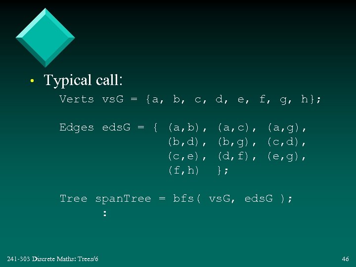• Typical call: Verts vs. G = {a, b, c, d, e, f, g, h}; Edges eds. G = { (a, b), (b, d), (c, e), (f, h) (a, c), (a, g), (b, g), (c, d), (d, f), (e, g), }; Tree span. Tree = bfs( vs. G, eds. G ); : 241 -303 Discrete Maths: Trees/6 46

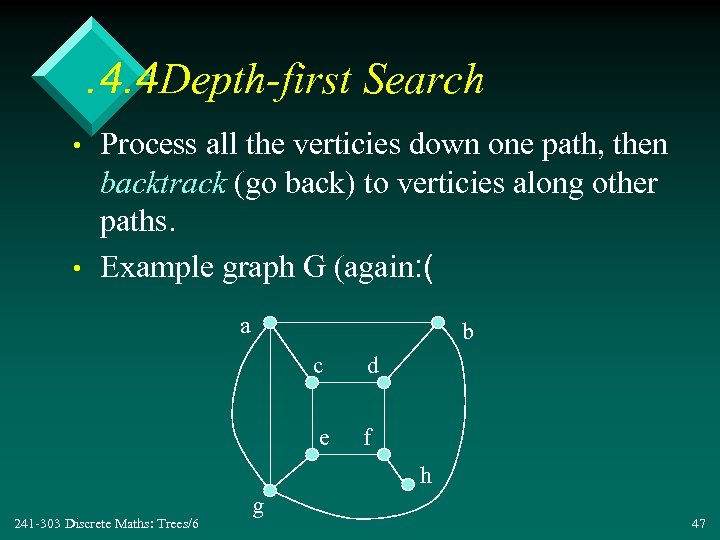. 4. 4 Depth-first Search • • Process all the verticies down one path, then backtrack (go back) to verticies along other paths. Example graph G (again: ( a b c d e f h 241 -303 Discrete Maths: Trees/6 g 47

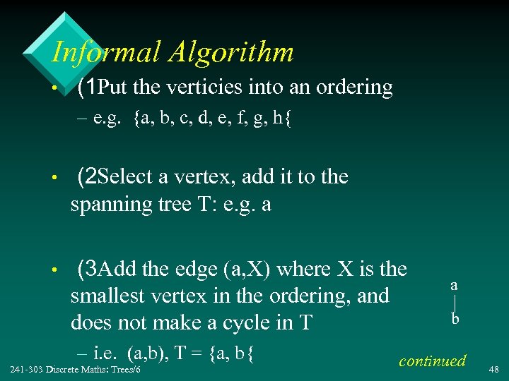Informal Algorithm • (1 Put the verticies into an ordering – e. g. {a, b, c, d, e, f, g, h{ • (2 Select a vertex, add it to the spanning tree T: e. g. a • (3 Add the edge (a, X) where X is the smallest vertex in the ordering, and does not make a cycle in T – i. e. (a, b), T = {a, b{ 241 -303 Discrete Maths: Trees/6 a b continued 48

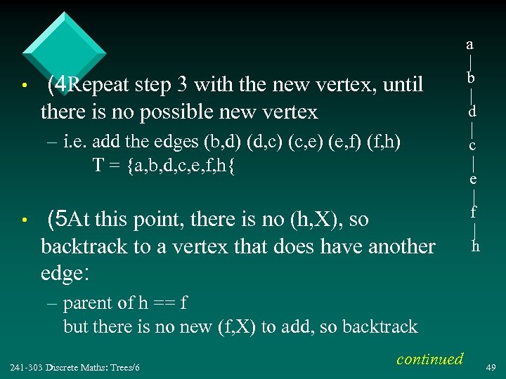a • (4 Repeat step 3 with the new vertex, until there is no possible new vertex – i. e. add the edges (b, d) (d, c) (c, e) (e, f) (f, h) T = {a, b, d, c, e, f, h{ • (5 At this point, there is no (h, X), so backtrack to a vertex that does have another edge: b d c e f h – parent of h == f but there is no new (f, X) to add, so backtrack 241 -303 Discrete Maths: Trees/6 continued 49

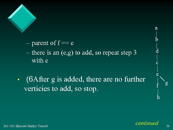a – parent of f == e – there is an (e, g) to add, so repeat step 3 with e • (6 After g is added, there are no further verticies to add, so stop. b d c e f g h 241 -303 Discrete Maths: Trees/6 continued 50

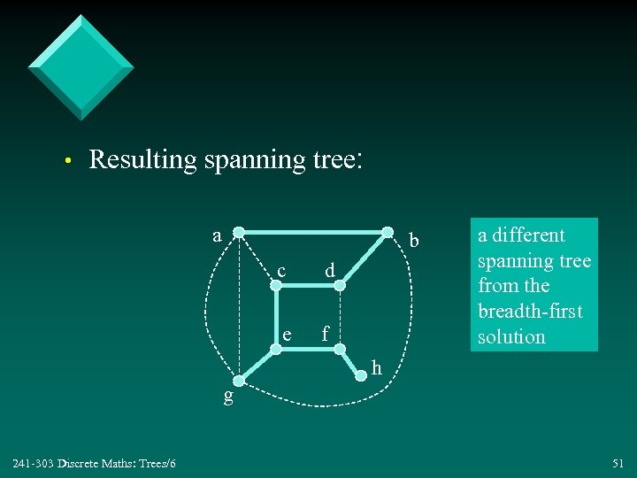• Resulting spanning tree: a b c d e f a different spanning tree from the breadth-first solution h g 241 -303 Discrete Maths: Trees/6 51

. 4. 5 Another Backtracking Problem Summing a Subset • Find a subset of {31, 27, 15, 11, 7, 5} with a sum that equals 39. – one answer is {27, 7, 5{ • How? : build up the sum by adding integers. An integer is included if the sum remains less than 39. – backtracking is required to try different integers when the sum doesn't reach 39. 241 -303 Discrete Maths: Trees/6 52

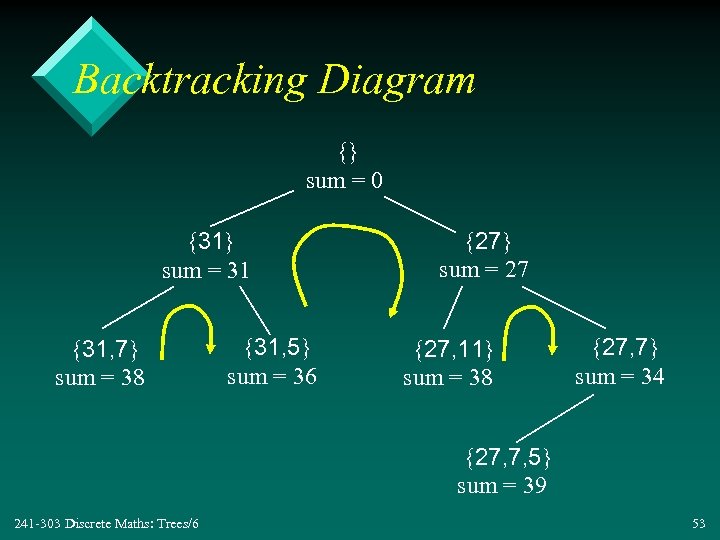Backtracking Diagram {} sum = 0 {31} sum = 31 {31, 7} sum = 38 {31, 5} sum = 36 {27} sum = 27 {27, 11} sum = 38 {27, 7} sum = 34 {27, 7, 5} sum = 39 241 -303 Discrete Maths: Trees/6 53

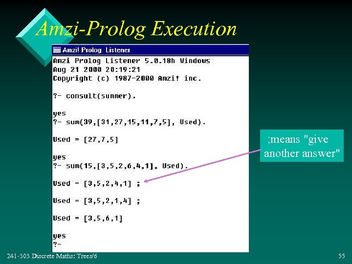
Prolog Code and Query • sum(0, _, []). sum(Sum, List, [X|Used]) : Sum > 0, select(List, X, List 1), Sum 1 is Sum - X, sum(Sum 1, List 1, Used). It can calculate sums of any set. select([X|L], X, L). select([Y|L], X, [Y|L 1]) : select(L, X, L 1. ( • -? sum(39, [31, 27, 15, 11, 7, 5], Used). Used = [27, 7, 5[ 241 -303 Discrete Maths: Trees/6 54

Amzi-Prolog Execution ; means "give another answer" 241 -303 Discrete Maths: Trees/6 55

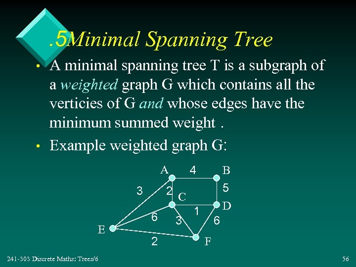. 5 Minimal Spanning Tree • • A minimal spanning tree T is a subgraph of a weighted graph G which contains all the verticies of G and whose edges have the minimum summed weight. Example weighted graph G: A 3 E 241 -303 Discrete Maths: Trees/6 4 B 5 D 2 C 6 2 3 1 6 F 56

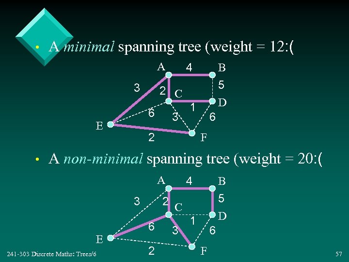• A minimal spanning tree (weight = 12: ( A 3 • B 5 D 2 C 6 E 4 3 1 2 6 F A non-minimal spanning tree (weight = 20: ( A 3 E 241 -303 Discrete Maths: Trees/6 4 B 5 D 2 C 6 2 3 1 6 F 57

. 5. 1 Prim's Algorithm • Prim's algorithm finds a minimal spanning tree T by iteratively adding edges to T. • At each iteration, a minimum-weight edge is added that does not create a cycle in the current T. 241 -303 Discrete Maths: Trees/6 58

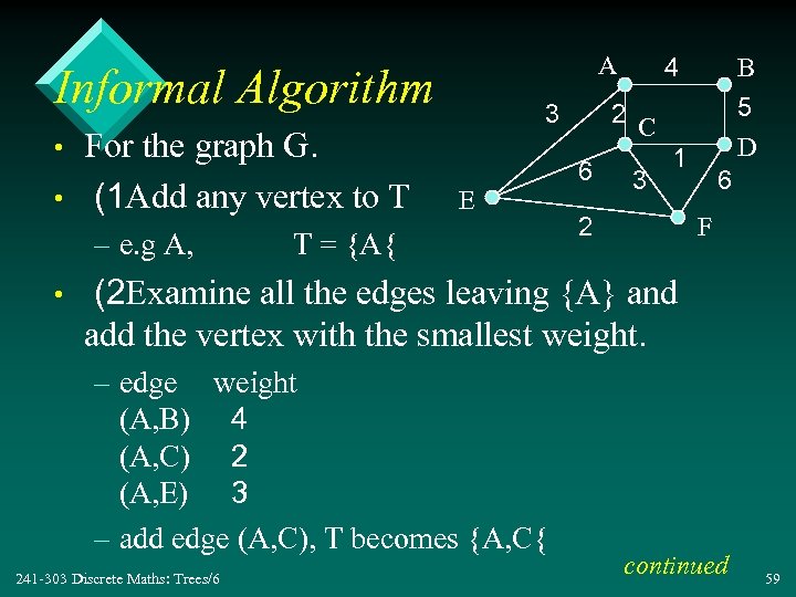A Informal Algorithm • • For the graph G. (1 Add any vertex to T – e. g A, • 3 E T = {A{ 4 B 5 D 2 C 6 3 1 2 6 F (2 Examine all the edges leaving {A} and add the vertex with the smallest weight. – edge weight (A, B) 4 (A, C) 2 (A, E) 3 – add edge (A, C), T becomes {A, C{ 241 -303 Discrete Maths: Trees/6 continued 59

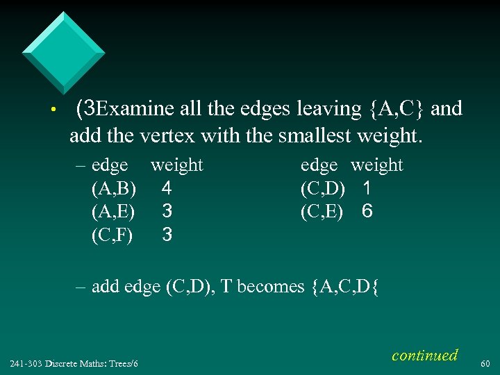• (3 Examine all the edges leaving {A, C} and add the vertex with the smallest weight. – edge weight (A, B) 4 (A, E) 3 (C, F) 3 edge weight (C, D) 1 (C, E) 6 – add edge (C, D), T becomes {A, C, D{ 241 -303 Discrete Maths: Trees/6 continued 60

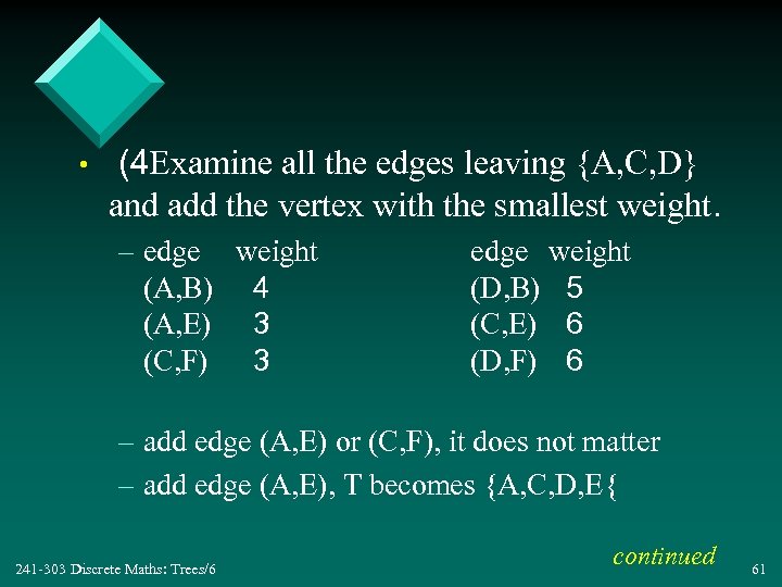• (4 Examine all the edges leaving {A, C, D} and add the vertex with the smallest weight. – edge weight (A, B) 4 (A, E) 3 (C, F) 3 edge weight (D, B) 5 (C, E) 6 (D, F) 6 – add edge (A, E) or (C, F), it does not matter – add edge (A, E), T becomes {A, C, D, E{ 241 -303 Discrete Maths: Trees/6 continued 61

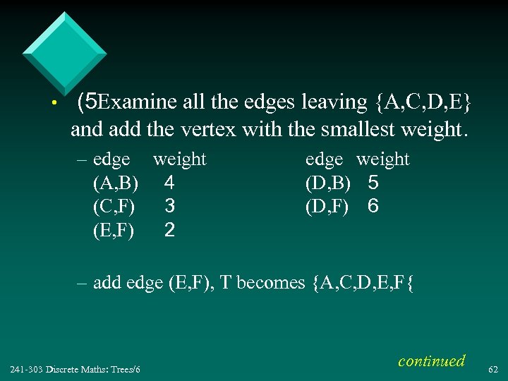• (5 Examine all the edges leaving {A, C, D, E} and add the vertex with the smallest weight. – edge weight (A, B) 4 (C, F) 3 (E, F) 2 edge weight (D, B) 5 (D, F) 6 – add edge (E, F), T becomes {A, C, D, E, F{ 241 -303 Discrete Maths: Trees/6 continued 62

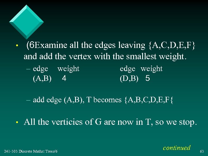• (6 Examine all the edges leaving {A, C, D, E, F} and add the vertex with the smallest weight. – edge weight (A, B) 4 edge weight (D, B) 5 – add edge (A, B), T becomes {A, B, C, D, E, F{ • All the verticies of G are now in T, so we stop. 241 -303 Discrete Maths: Trees/6 continued 63

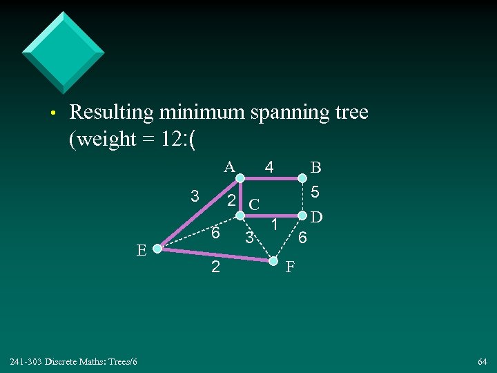• Resulting minimum spanning tree (weight = 12: ( A 3 E 241 -303 Discrete Maths: Trees/6 4 B 5 D 2 C 6 2 3 1 6 F 64

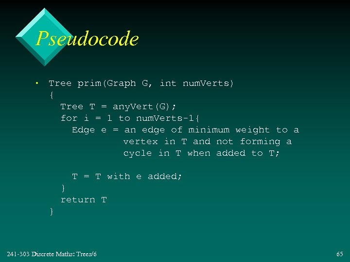Pseudocode • Tree prim(Graph G, int num. Verts) { Tree T = any. Vert(G); for i = 1 to num. Verts-1{ Edge e = an edge of minimum weight to a vertex in T and not forming a cycle in T when added to T; T = T with e added; } return T } 241 -303 Discrete Maths: Trees/6 65

. 5. 2 A Greedy Algorithm • Prim's algorithm is an example of a greedy algorithm – its choice at each iteration does not depend on any previous choices • A greedy algorithm does the best thing at this time without considering the past (or the future. ( 241 -303 Discrete Maths: Trees/6 66

Greed is not Always Best • An example where greed is not the best approach: – a greedy shortest-path algorithm can lead to a non-optimal solution (not the best( – the algorithm selects an edge with the minimum weight connected to the last vertex added 241 -303 Discrete Maths: Trees/6 continued 67

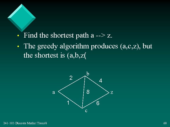• • Find the shortest path a --> z. The greedy algorithm produces (a, c, z), but the shortest is (a, b, z( 2 b 4 8 a 1 z 6 c 241 -303 Discrete Maths: Trees/6 68

. 5. 3 Kruskal's Minimum Spanning Tree Algorithm • At the start, the minimum spanning tree T consists of all the verticies of the weighted graph G, but no edges. • At each iteration, add an edge e to T having minimum weight that does not create a cycle in T. • When T has n-1 edges, stop. 241 -303 Discrete Maths: Trees/6 69

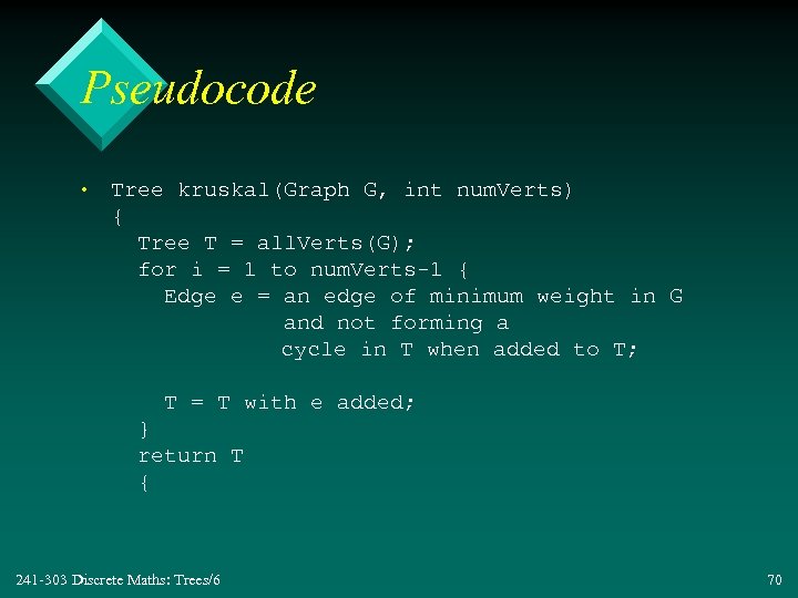Pseudocode • Tree kruskal(Graph G, int num. Verts) { Tree T = all. Verts(G); for i = 1 to num. Verts-1 { Edge e = an edge of minimum weight in G and not forming a cycle in T when added to T; T = T with e added; } return T { 241 -303 Discrete Maths: Trees/6 70

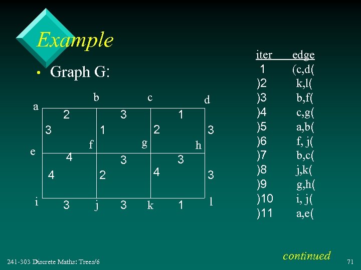Example • Graph G: b a 2 e 1 4 d 3 3 1 2 g f 4 2 3 j 241 -303 Discrete Maths: Trees/6 3 3 h 3 4 i c k 3 3 1 l iter 1 )2 )3 )4 )5 )6 )7 )8 )9 )10 )11 edge (c, d( k, l( b, f( c, g( a, b( f, j( b, c( j, k( g, h( i, j( a, e( continued 71

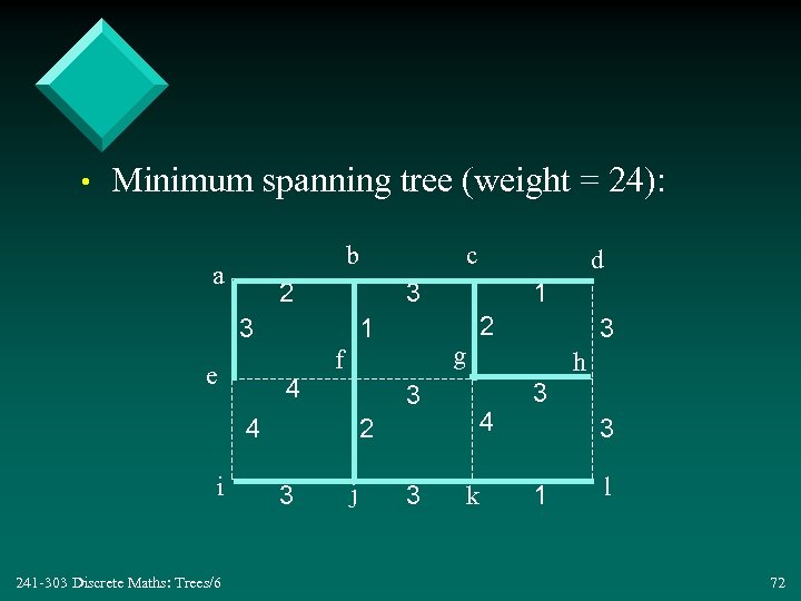• Minimum spanning tree (weight = 24): b a 2 e 1 4 1 2 g f 4 2 3 j 3 3 h 3 4 241 -303 Discrete Maths: Trees/6 d 3 3 i c k 3 3 1 l 72

. 5. 4 Difference between Prim and Kruskal • Prim's algorithm chooses an edge that must already be connected to a vertex in the minimum spanning tree T. • Kruskal's algorithm can choose an edge that may not already be connected to a vertex in T. 241 -303 Discrete Maths: Trees/6 73

. 6 Game Trees • Trees can be used to develop game-playing strategies – used in many AI (Artificial Intelligence) game programs where the human is competing against the 'clever' machine 241 -303 Discrete Maths: Trees/6 74

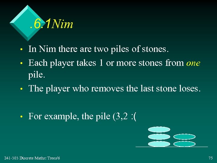. 6. 1 Nim • In Nim there are two piles of stones. Each player takes 1 or more stones from one pile. The player who removes the last stone loses. • For example, the pile (3, 2 : ( • • 241 -303 Discrete Maths: Trees/6 75

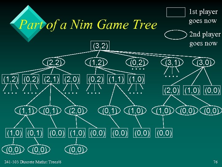1 st player goes now Part of a Nim Game Tree 2 nd player goes now (3, 2) (2, 2) (1, 2) (0, 2). . (1, 2) (0, 2) (2, 1) (2, 0) (0, 2) (1, 1) (1, 0) . . . (1, 1) . . (0, 1) (2, 0) . . (0, 1) (1, 0) (3, 1) (3, 0) . . (2, 0) (1, 0) (0, 0) (1, 0) (0, 1) (0, 0) (1, 0) (0, 0) (0, 0) 241 -303 Discrete Maths: Trees/6 (0, 0) 76

Analysing the Game Tree • Label each terminal vertex with the first player's score: – if the first player won, write "1" – if the first player lost, write "0" 241 -303 Discrete Maths: Trees/6 continued 77

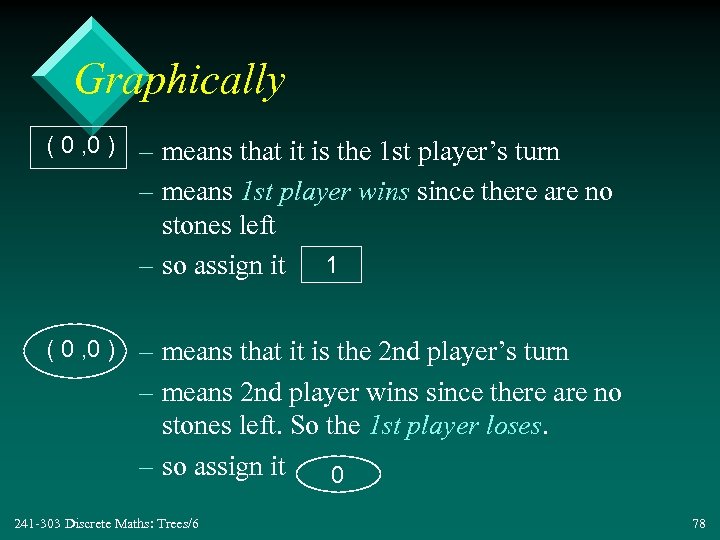Graphically ( 0 , 0 ) – means that it is the 1 st player’s turn – means 1 st player wins since there are no stones left – so assign it 1 ( 0 , 0 ) – means that it is the 2 nd player’s turn – means 2 nd player wins since there are no stones left. So the 1 st player loses. – so assign it 0 241 -303 Discrete Maths: Trees/6 78

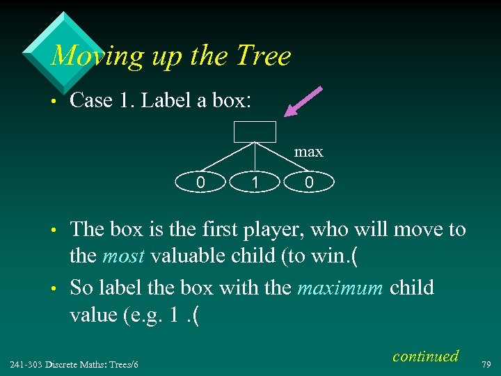Moving up the Tree • Case 1. Label a box: max 0 • • 1 0 The box is the first player, who will move to the most valuable child (to win. ( So label the box with the maximum child value (e. g. 1. ( 241 -303 Discrete Maths: Trees/6 continued 79

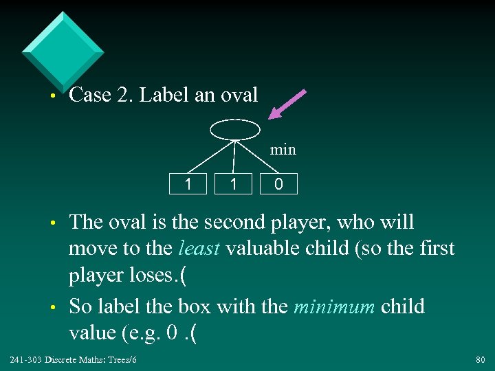• Case 2. Label an oval min 1 • • 1 0 The oval is the second player, who will move to the least valuable child (so the first player loses. ( So label the box with the minimum child value (e. g. 0. ( 241 -303 Discrete Maths: Trees/6 80

The Minimax Algorithm • In many games: – the first player chooses the most valuable position to move to; and – the second player chooses the least valuable position for the first player • The minimax algorithm: – first player seeks the max of the child values – second player seeks the min of the child values 241 -303 Discrete Maths: Trees/6 81

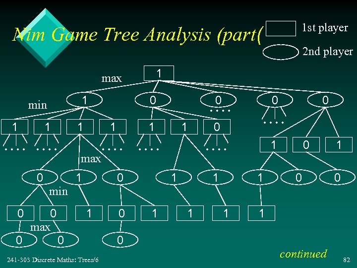1 st player Nim Game Tree Analysis (part( 1 max 1 min 1 1 1 . . . . 0 0 1 max 1 2 nd player 1 . . 0. . . . 0 1 0 0. . . . 1 1 0 0 1 0 min 0 0 0 max 1 0 241 -303 Discrete Maths: Trees/6 0 1 1 0 continued 82

• The root value (the starting position) contains a "1" – this means that the first player will definitely win if he/she chooses the most valuable child position to move to 241 -303 Discrete Maths: Trees/6 83

Larger Game Trees • Games like Chess or Go generate game trees that are too large to analyse using a simple minimax algorithm. • Instead the game tree is generated to a certain level, and then an evaluation function is used to 'calculate' the scores at that level for the first player. • Minimax is then used to work back to the root. 241 -303 Discrete Maths: Trees/6 84

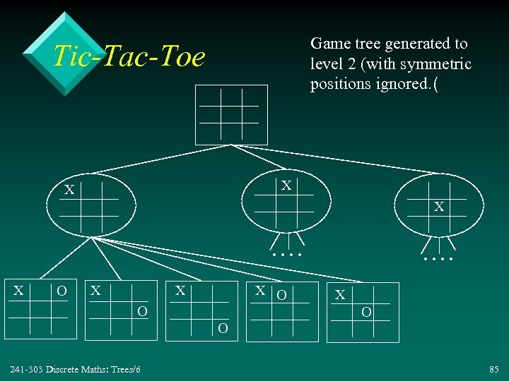Game tree generated to level 2 (with symmetric positions ignored. ( Tic-Tac-Toe X X X . . X O X X X O O . . X O O 241 -303 Discrete Maths: Trees/6 85

The Evaluation Function • For a given position P: – eval(P) = num. Wins. X - num. Wins. O; – num. Wins. X = number of rows, columns, and diagonals containing an X that the X player might be able to complete in the future – num. Wins. O = same, but for O 241 -303 Discrete Maths: Trees/6 continued 86

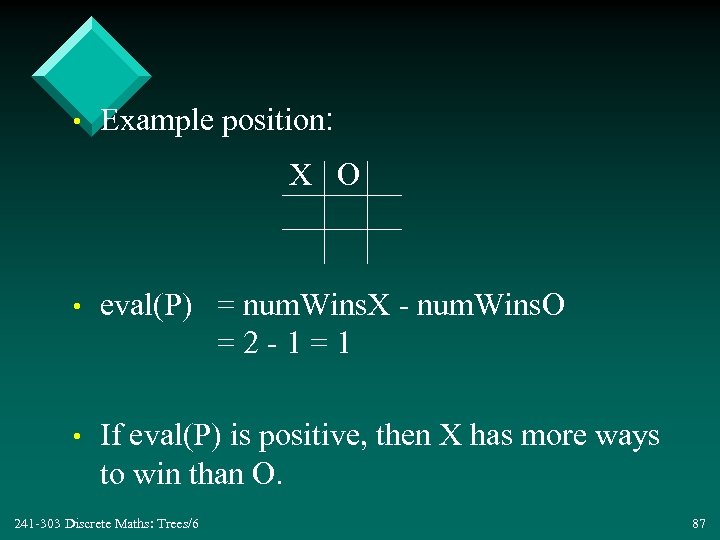• Example position: X O • eval(P) = num. Wins. X - num. Wins. O =2 -1=1 • If eval(P) is positive, then X has more ways to win than O. 241 -303 Discrete Maths: Trees/6 87

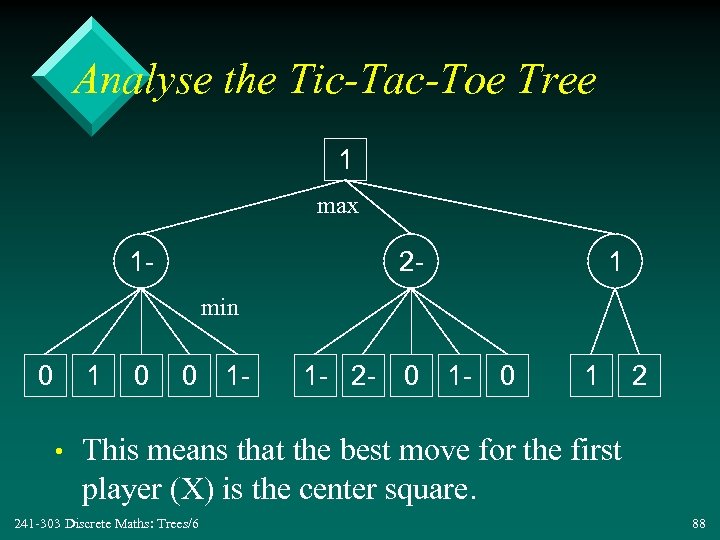Analyse the Tic-Tac-Toe Tree 1 max 1 - 2 - 1 min 0 1 • 0 0 1 - 1 - 2 - 0 1 2 This means that the best move for the first player (X) is the center square. 241 -303 Discrete Maths: Trees/6 88

Alpha-Beta Pruning • Evaluating a game tree with a large level takes too much time. • Alpha-beta pruning reduces the number of positions (verticies) that need to be evaluated, and still gives the right answer. • There are two parts to alpha-beta pruning: – alpha cutoff – beta cutoff 241 -303 Discrete Maths: Trees/6 89

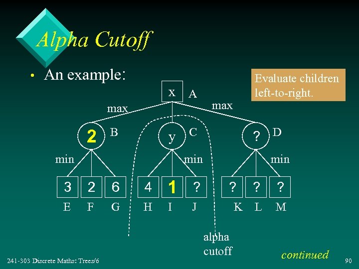Alpha Cutoff • An example: x A max 2 B Evaluate children left-to-right. max y C min ? D min 3 2 6 4 1 ? E F G H I min J 241 -303 Discrete Maths: Trees/6 ? K alpha cutoff ? ? L M continued 90

• In A, x must be >= 2 – the lower bound for A, the alpha value for A • In C, y must be <= 1 – since y <= x, it cannot affect x, so there is no need to evaluate J – also the C subtree can be ignored (cutoff( • Alpha cutoff occurs when a grandchild of A (e. g. I) has a value <= the alpha value of A. 241 -303 Discrete Maths: Trees/6 91

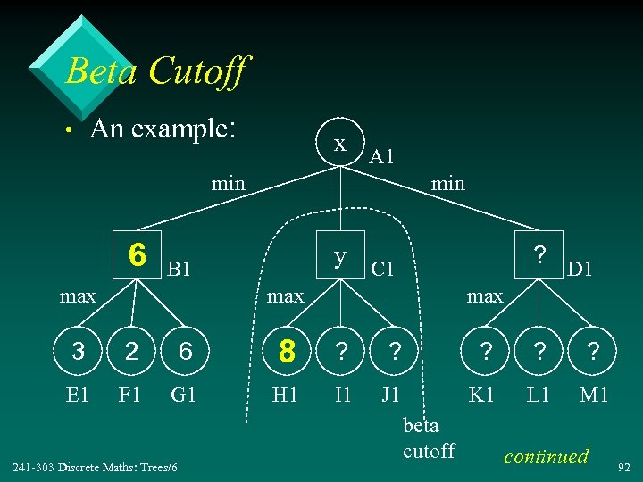Beta Cutoff • An example: x A 1 min 6 min B 1 max ? D 1 y C 1 max 3 2 6 8 ? ? ? E 1 F 1 G 1 H 1 I 1 J 1 K 1 L 1 M 1 241 -303 Discrete Maths: Trees/6 beta cutoff continued 92

• In A 1, x must be <= 6 – the upper bound for A 1, the beta value for A 1 • In C 1, y must be >= 8 – since y >= x, it cannot affect x, so there is no need to evaluate I 1 or J 1 – also the C 1 subtree can be ignored (cutoff( • Beta cutoff occurs when a grandchild of A 1 (e. g. H 1) has a value >= the beta value of A 1. 241 -303 Discrete Maths: Trees/6 93

. 7 More Information • DM: chapter 7 • Rosen: chapter 8 241 -303 Discrete Maths: Trees/6 94