Discrete Mathematics CS 2610 1 Propositional Logic

Discrete Mathematics CS 2610 1

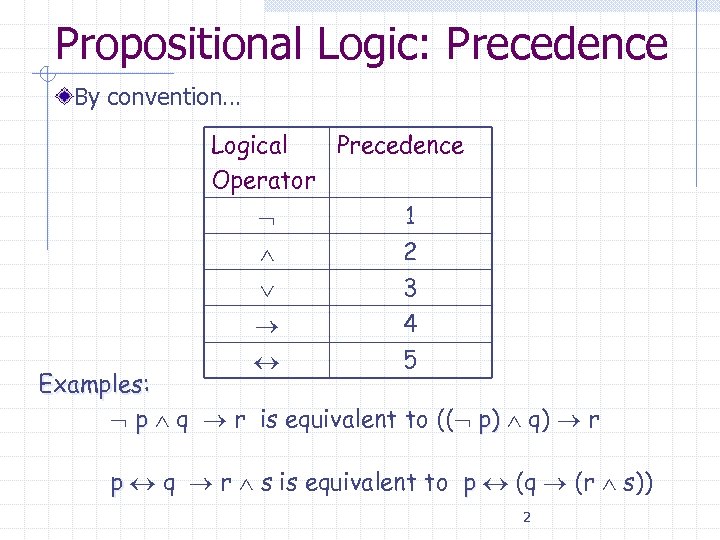Propositional Logic: Precedence By convention… Logical Precedence Operator 1 2 3 4 5 Examples: p q r is equivalent to (( p) q) r p q r s is equivalent to p (q (r s)) 2

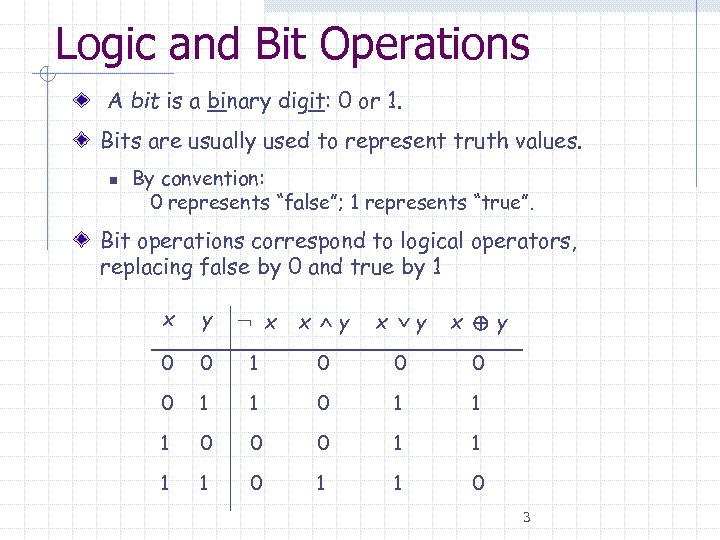Logic and Bit Operations A bit is a binary digit: 0 or 1. Bits are usually used to represent truth values. n By convention: 0 represents “false”; 1 represents “true”. Bit operations correspond to logical operators, replacing false by 0 and true by 1 x y x x y x y 0 0 1 1 0 1 1 1 0 0 0 1 1 0 3

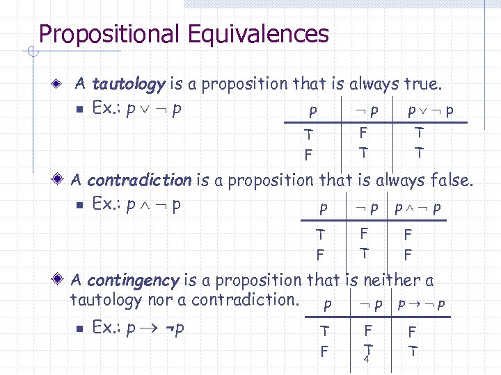Propositional Equivalences A tautology is a proposition that is always true. n Ex. : p p p T T F A contradiction is a proposition that is always false. n Ex. : p p p T F F A contingency is a proposition that is neither a tautology nor a contradiction. p p n Ex. : p ¬p T F F T 4 F T

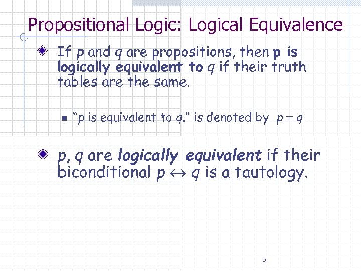Propositional Logic: Logical Equivalence If p and q are propositions, then p is logically equivalent to q if their truth tables are the same. n “p is equivalent to q. ” is denoted by p q p, q are logically equivalent if their biconditional p q is a tautology. 5

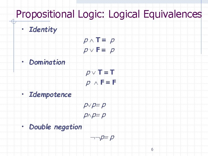Propositional Logic: Logical Equivalences • Identity p T p p F p • Domination p T T p F F • Idempotence p p p • Double negation p p 6

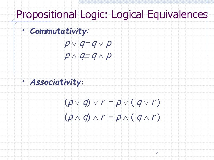Propositional Logic: Logical Equivalences • Commutativity: p q q p • Associativity: (p q) r p ( q r ) 7

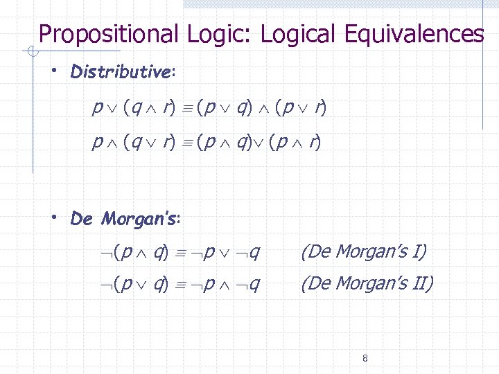Propositional Logic: Logical Equivalences • Distributive: p (q r) (p q) (p r) p (q r) (p q) (p r) • De Morgan’s: (p q) p q (De Morgan’s I) (p q) p q (De Morgan’s II) 8

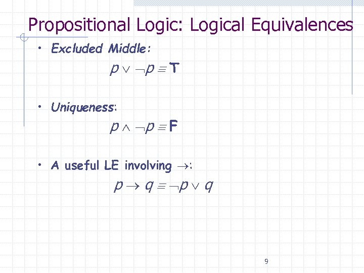Propositional Logic: Logical Equivalences • Excluded Middle: p p T • Uniqueness: p p F • A useful LE involving : p q 9

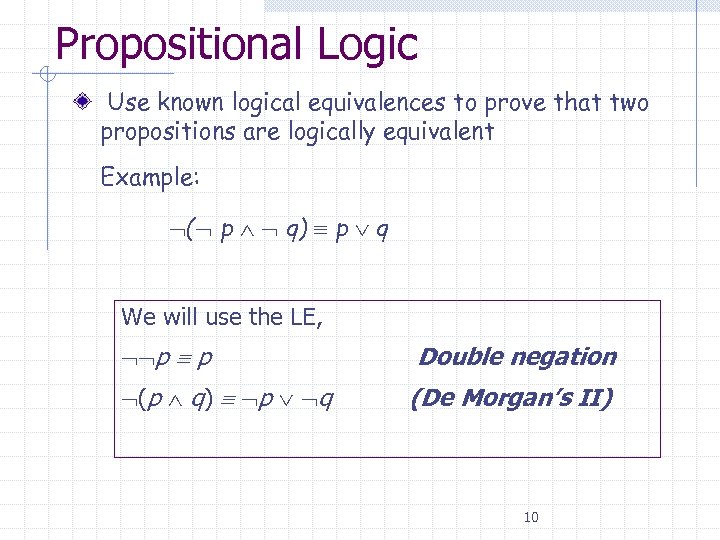Propositional Logic Use known logical equivalences to prove that two propositions are logically equivalent Example: ( p q) p q We will use the LE, p p (p q) p q Double negation (De Morgan’s II) 10

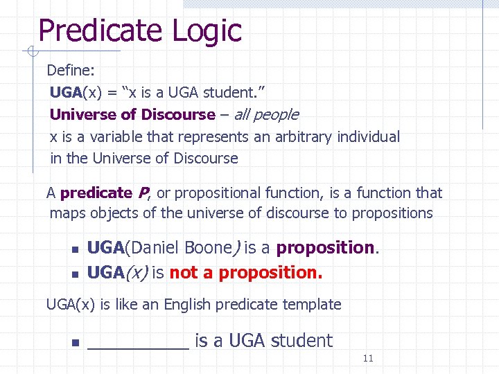Predicate Logic Define: UGA(x) = “x is a UGA student. ” Universe of Discourse – all people x is a variable that represents an arbitrary individual in the Universe of Discourse A predicate P, or propositional function, is a function that maps objects of the universe of discourse to propositions n n UGA(Daniel Boone) is a proposition. UGA(x) is not a proposition. UGA(x) is like an English predicate template n _____ is a UGA student 11

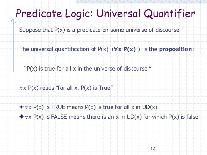Predicate Logic: Universal Quantifier Suppose that P(x) is a predicate on some universe of discourse. The universal quantification of P(x) ( x P(x) ) is the proposition: “P(x) is true for all x in the universe of discourse. ” x P(x) reads “for all x, P(x) is True” x P(x) is TRUE means P(x) is true for all x in UD(x). x P(x) is FALSE means there is an x in UD(x) for which P(x) is false. 12

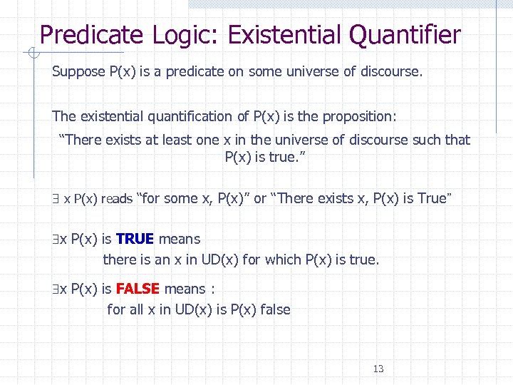Predicate Logic: Existential Quantifier Suppose P(x) is a predicate on some universe of discourse. The existential quantification of P(x) is the proposition: “There exists at least one x in the universe of discourse such that P(x) is true. ” x P(x) reads “for some x, P(x)” or “There exists x, P(x) is True” x P(x) is TRUE means there is an x in UD(x) for which P(x) is true. x P(x) is FALSE means : for all x in UD(x) is P(x) false 13

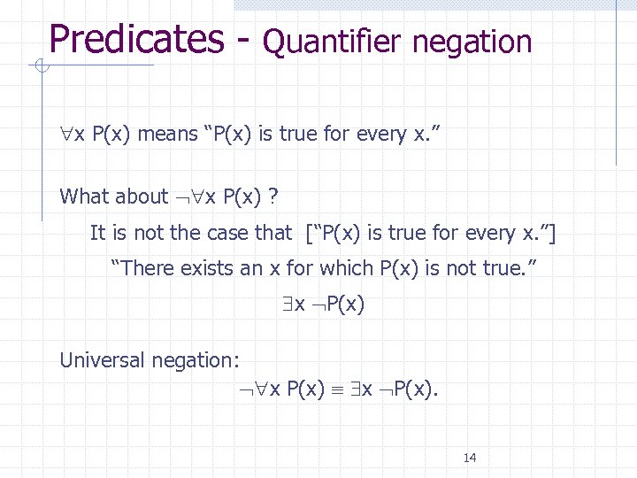Predicates - Quantifier negation x P(x) means “P(x) is true for every x. ” What about x P(x) ? It is not the case that [“P(x) is true for every x. ”] “There exists an x for which P(x) is not true. ” x P(x) Universal negation: x P(x). 14

Proofs • A theorem is a statement that can be proved to be true. • A proof is a sequence of statements that form an argument. 15

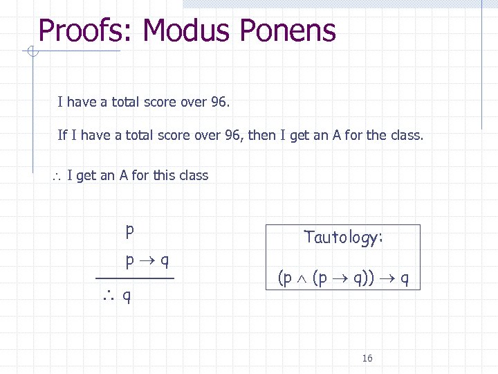Proofs: Modus Ponens • I have a total score over 96. • If I have a total score over 96, then I get an A for the class. I get an A for this class p p q q Tautology: (p q)) q 16

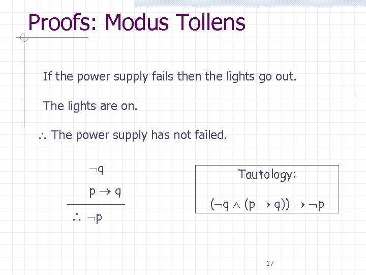Proofs: Modus Tollens • If the power supply fails then the lights go out. • The lights are on. The power supply has not failed. q p Tautology: ( q (p q)) p 17

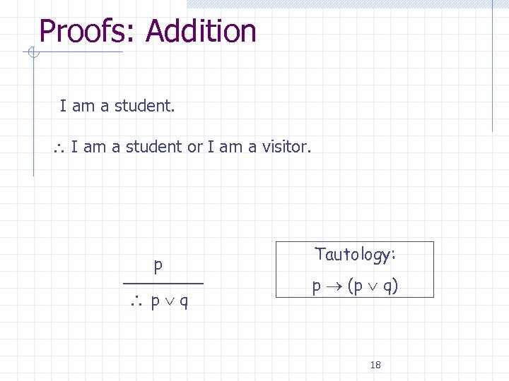Proofs: Addition • I am a student or I am a visitor. p p q Tautology: p (p q) 18

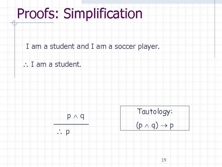Proofs: Simplification • I am a student and I am a soccer player. I am a student. p q p Tautology: (p q) p 19

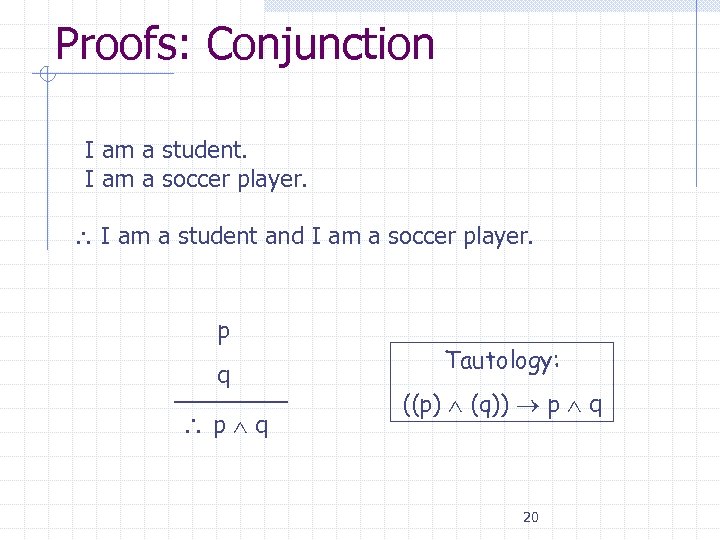Proofs: Conjunction • I am a student. • I am a soccer player. I am a student and I am a soccer player. p q p q Tautology: ((p) (q)) p q 20

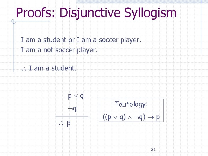Proofs: Disjunctive Syllogism I am a student or I am a soccer player. I am a not soccer player. I am a student. p q q p Tautology: ((p q) p 21

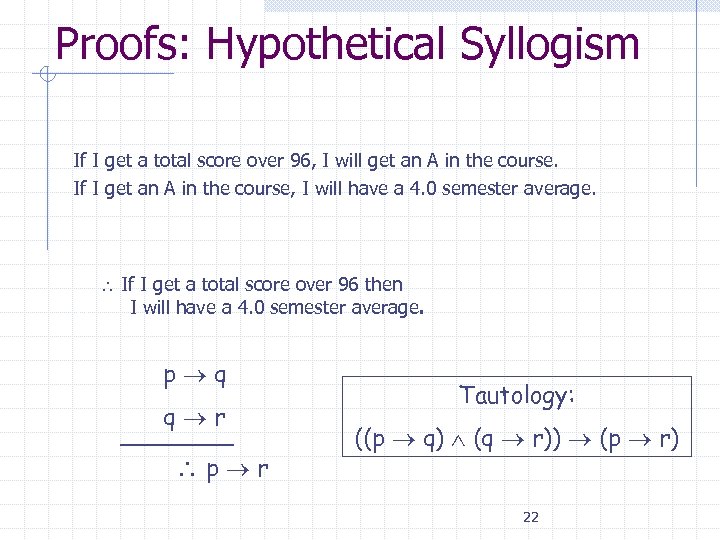Proofs: Hypothetical Syllogism If I get a total score over 96, I will get an A in the course. If I get an A in the course, I will have a 4. 0 semester average. If I get a total score over 96 then I will have a 4. 0 semester average. p q q r p r Tautology: ((p q) (q r)) (p r) 22

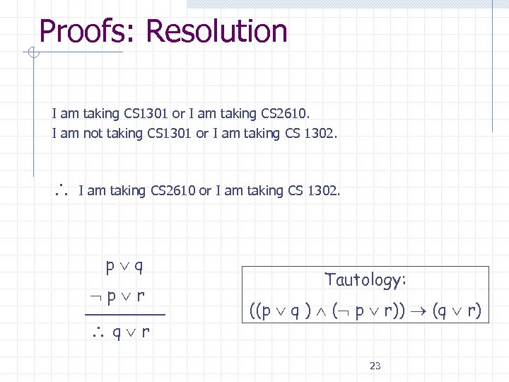Proofs: Resolution I am taking CS 1301 or I am taking CS 2610. I am not taking CS 1301 or I am taking CS 1302. I am taking CS 2610 or I am taking CS 1302. p q p r q r Tautology: ((p q ) ( p r)) (q r) 23

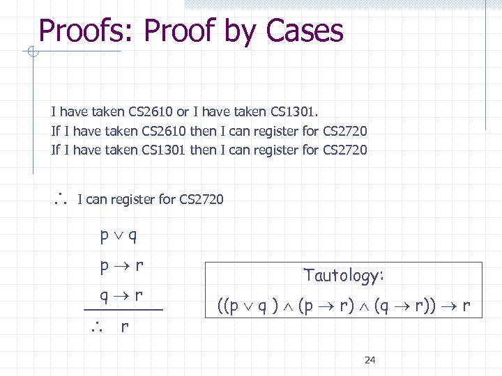Proofs: Proof by Cases I have taken CS 2610 or I have taken CS 1301. If I have taken CS 2610 then I can register for CS 2720 If I have taken CS 1301 then I can register for CS 2720 p q p r q r r Tautology: ((p q ) (p r) (q r)) r 24

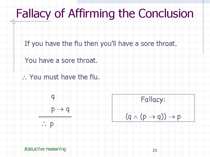Fallacy of Affirming the Conclusion • If you have the flu then you’ll have a sore throat. • You have a sore throat. You must have the flu. q p q p Abductive reasoning Fallacy: (q (p q)) p 25

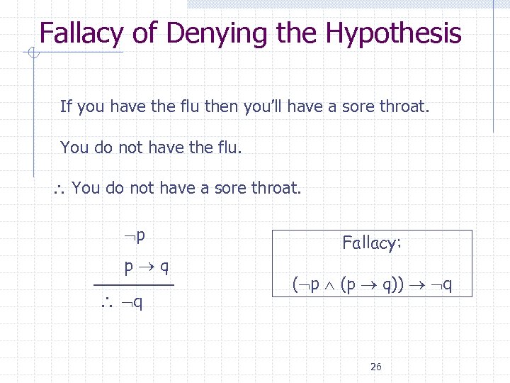Fallacy of Denying the Hypothesis • If you have the flu then you’ll have a sore throat. • You do not have the flu. You do not have a sore throat. p p q q Fallacy: ( p (p q)) q 26

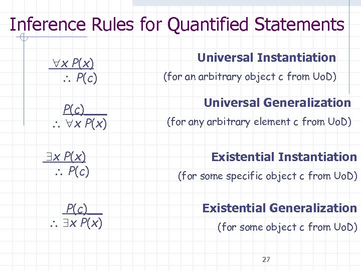Inference Rules for Quantified Statements x P(x) P(c)___ x P(x) P(c)__ x P(x) Universal Instantiation (for an arbitrary object c from Uo. D) Universal Generalization (for any arbitrary element c from Uo. D) Existential Instantiation (for some specific object c from Uo. D) Existential Generalization (for some object c from Uo. D) 27

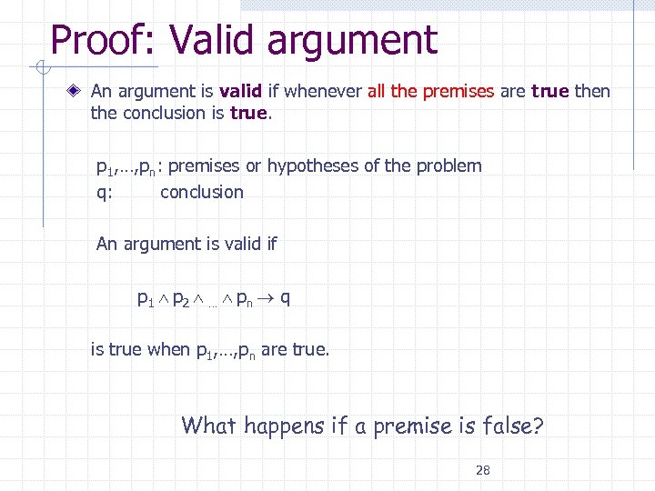Proof: Valid argument An argument is valid if whenever all the premises are true then the conclusion is true. p 1, …, pn: premises or hypotheses of the problem q: conclusion An argument is valid if p 1 p 2 … pn q is true when p 1, …, pn are true. What happens if a premise is false? 28

Proofs Step 1: Translate the sentences into logical expressions Step 2: Use rules of inferences to build a proof 29

Direct proofs Start with premises and deduce the conclusion: n n Assume that the premises are true Apply rules of inferences and theorems 30

Vacuous Proofs p q is vacuously true if p is false In this case, p q is a vacuous proof Ex. p: 0 > 1 q: Mars is an asteroid What can we say about p q ? 31

Trivial Proofs p q is trivially true if q is true, In this case, we have a trivial proof Example: x>1 1=1 32

Indirect Proofs To prove p q, we prove its contrapositive, q p Example: if n 2 is even then n is even is equivalent to … if n is odd then n 2 is odd We can prove “If n 2 is even then n is even” by proving “If n is odd then n 2 is odd” 33

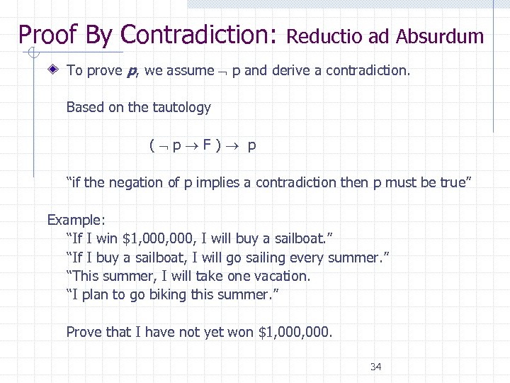Proof By Contradiction: Reductio ad Absurdum To prove p, we assume p and derive a contradiction. Based on the tautology ( p F ) p “if the negation of p implies a contradiction then p must be true” Example: “If I win $1, 000, I will buy a sailboat. ” “If I buy a sailboat, I will go sailing every summer. ” “This summer, I will take one vacation. “I plan to go biking this summer. ” Prove that I have not yet won $1, 000. 34

Overview of last class A predicate P, or propositional function, is a function that maps objects in the universe of discourse to propositions Predicates can be quantified using the universal quantifier (“for all”) or the existential quantifier (“there exists”) Quantified predicates can be negated as follows n x P(x) Quantified variables are called “bound” Variables that are not quantified are called “free” 35

Proof Techniques-Quantifiers: For all Proofs x P(x) : provide a proof, not just examples. Ex. “The product of any two odd integers is odd” Proof: 36

Proof Techniques Disproving x P(x) n Find an counterexample for x P(x) w a value k in the Universe of Discourse such that P(k) n 2 Example: For every n positive number, 2 + 1 is prime. Find a counterexample: 37

Proof Techniques-Quantifiers: Existence Proofs Two ways of proving x P(x). Existence Constructive Proof: Find a k in the Uo. D such that P(k) holds. Existence Non-Constructive Proof Prove that x P(x) is true without finding a k in the Uo. D such that P(k) holds 38

Proof Techniques-Quantifiers: Existence Proofs x P(x) : Existence Constructive Proof: Find a k in the Uo. D such that P(k) holds. Example: There is a rational number that lies strictly between 19 100 - 1 and 19 100 Proof: 39

Existential Proof: Non-Constructive Prove that n N, p such that p is prime, and p > n. Proof: (BWOC) Assume the opposite is true. Then n, p such that p is prime, p n. Let p 1, p 2, …, pk be all the prime numbers between 2 and n. Consider the value r = p 1 × p 2 × … × pn + 1. Then r is not divisible by any prime number p n. Thus, either r is prime or r has prime factors greater than n! 40

Sets A set is an unordered collection of objects. Examples: { 1, 6, 7, 2, 9 } { a, d, e, 1, 2, 3} Order and repetition don’t matter = {6, 7, 1, 2, 9} = {a, a, d, d, e, e, 1, 2, 3} The empty set, or the set containing no elements. Note: { } = {} Singleton is a set S that contains exactly one element 41

Universal Set is the set containing all the objects under consideration. It is denoted by U 42

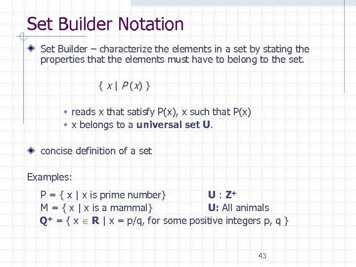Set Builder Notation Set Builder – characterize the elements in a set by stating the properties that the elements must have to belong to the set. { x | P (x) } w reads x that satisfy P(x), x such that P(x) w x belongs to a universal set U. concise definition of a set Examples: P = { x | x is prime number} U : Z+ M = { x | x is a mammal} U: All animals Q+ = { x R | x = p/q, for some positive integers p, q } 43

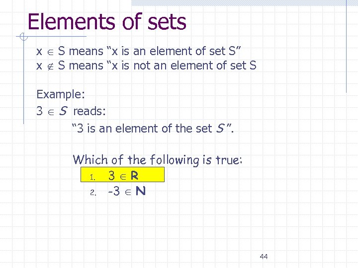Elements of sets x S means “x is an element of set S” x S means “x is not an element of set S Example: 3 S reads: “ 3 is an element of the set S ”. Which of the following is true: 1. 3 R 2. -3 N 44

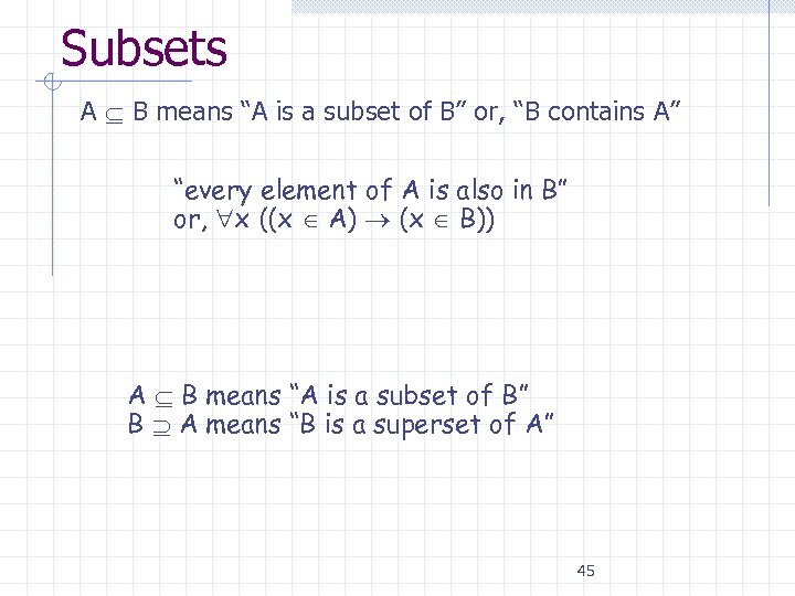Subsets A B means “A is a subset of B” or, “B contains A” “every element of A is also in B” or, x ((x A) (x B)) A B means “A is a subset of B” B A means “B is a superset of A” 45

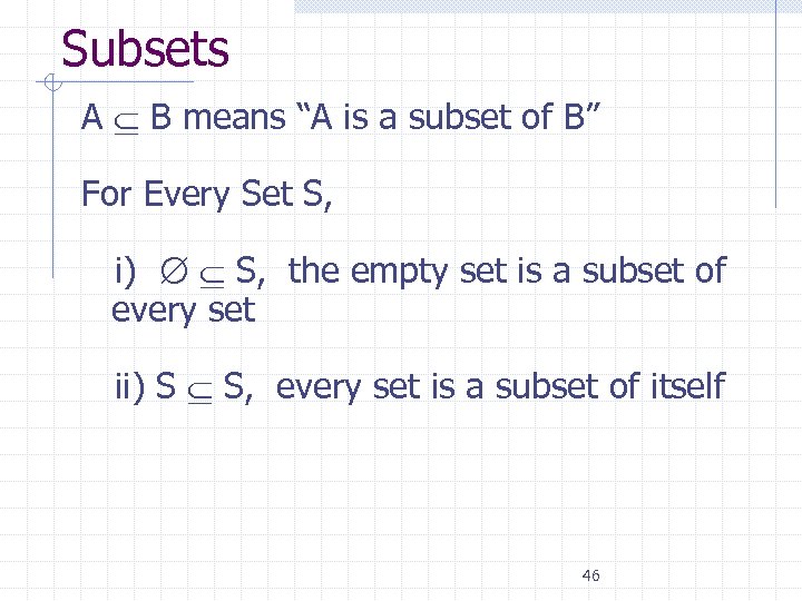Subsets A B means “A is a subset of B” For Every Set S, i) S, the empty set is a subset of every set ii) S S, every set is a subset of itself 46

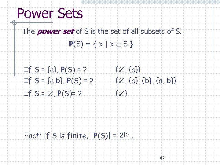Power Sets The power set of S is the set of all subsets of S. P(S) = { x | x S } If S = {a}, P(S) = ? If S = {a, b}, P(S) = ? { , {a}} { , {a}, {b}, {a, b}} If S = , P(S)= ? { } Fact: if S is finite, |P(S)| = 2|S|. 47

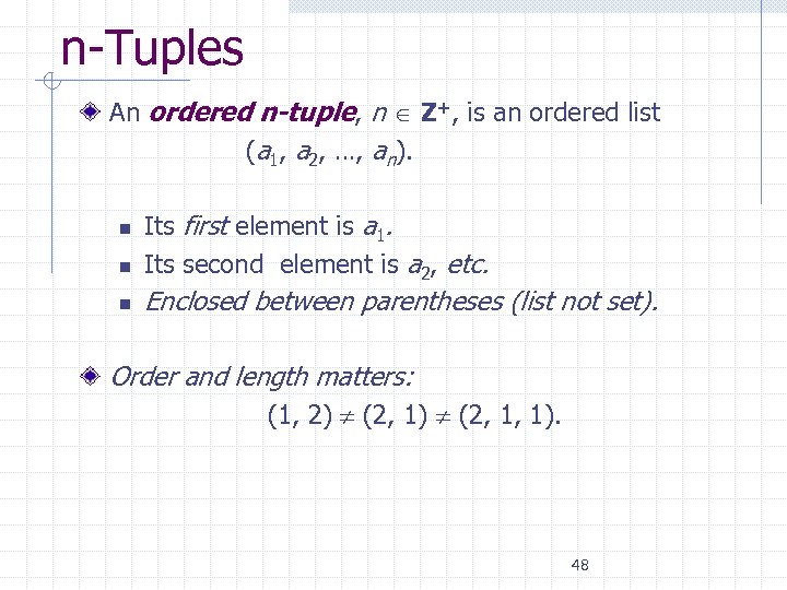n-Tuples An ordered n-tuple, n Z+, is an ordered list (a 1, a 2, …, an). n n n Its first element is a 1. Its second element is a 2, etc. Enclosed between parentheses (list not set). Order and length matters: (1, 2) (2, 1, 1). 48

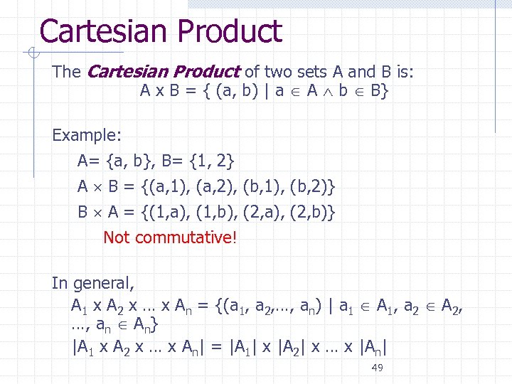Cartesian Product The Cartesian Product of two sets A and B is: A x B = { (a, b) | a A b B} Example: A= {a, b}, B= {1, 2} A B = {(a, 1), (a, 2), (b, 1), (b, 2)} B A = {(1, a), (1, b), (2, a), (2, b)} Not commutative! In general, A 1 x A 2 x … x An = {(a 1, a 2, …, an) | a 1 A 1, a 2 A 2, …, an An} |A 1 x A 2 x … x An| = |A 1| x |A 2| x … x |An| 49

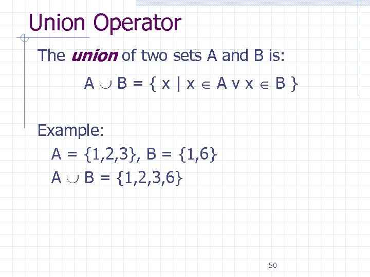Union Operator The union of two sets A and B is: A B = { x | x A v x B } Example: A = {1, 2, 3}, B = {1, 6} A B = {1, 2, 3, 6} 50

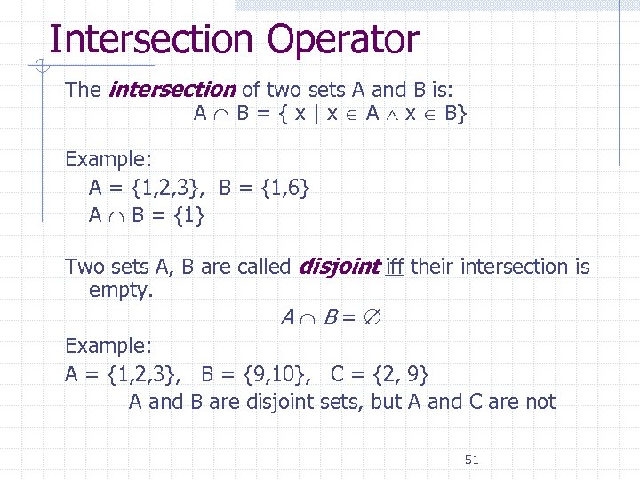Intersection Operator The intersection of two sets A and B is: A B = { x | x A x B} Example: A = {1, 2, 3}, B = {1, 6} A B = {1} Two sets A, B are called disjoint iff their intersection is empty. A B = Example: A = {1, 2, 3}, B = {9, 10}, C = {2, 9} A and B are disjoint sets, but A and C are not 51

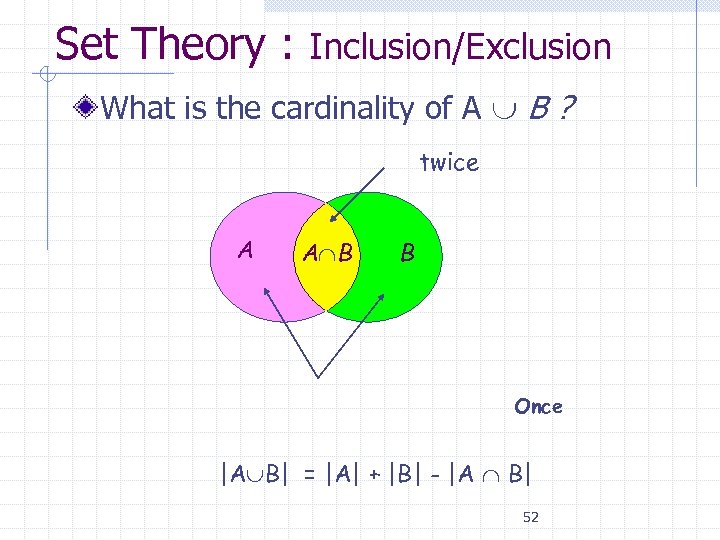Set Theory : Inclusion/Exclusion What is the cardinality of A B ? twice A A B B Once |A B| = |A| + |B| - |A B| 52

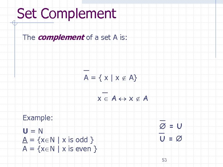Set Complement The complement of a set A is: A = { x | x A} x A Example: U = N A = {x N | x is odd } A = {x N | x is even } = U U = 53

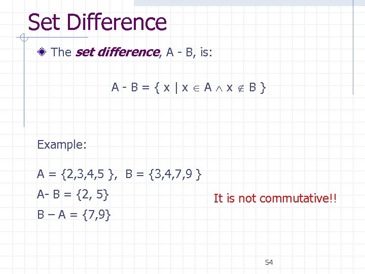Set Difference The set difference, A - B, is: A - B = { x | x A x B } Example: A = {2, 3, 4, 5 }, B = {3, 4, 7, 9 } A- B = {2, 5} It is not commutative!! B – A = {7, 9} 54

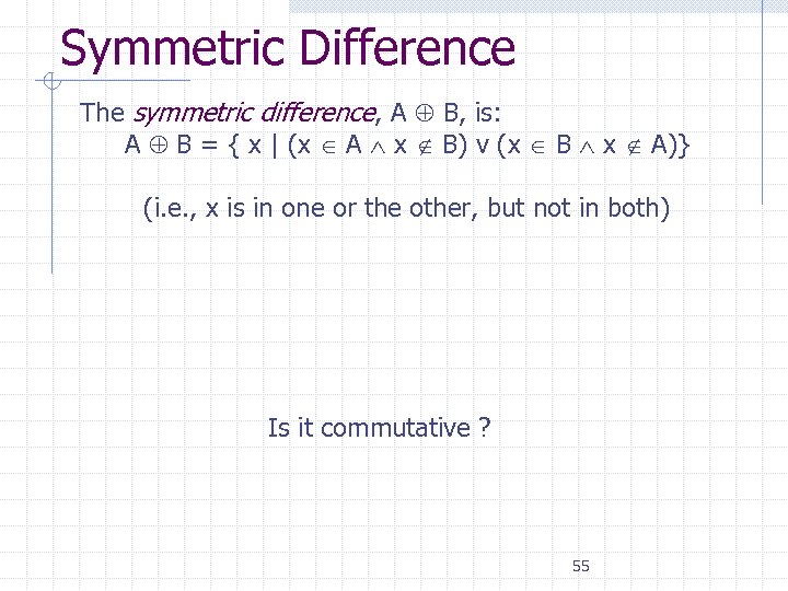Symmetric Difference The symmetric difference, A B, is: A B = { x | (x A x B) v (x B x A)} (i. e. , x is in one or the other, but not in both) Is it commutative ? 55

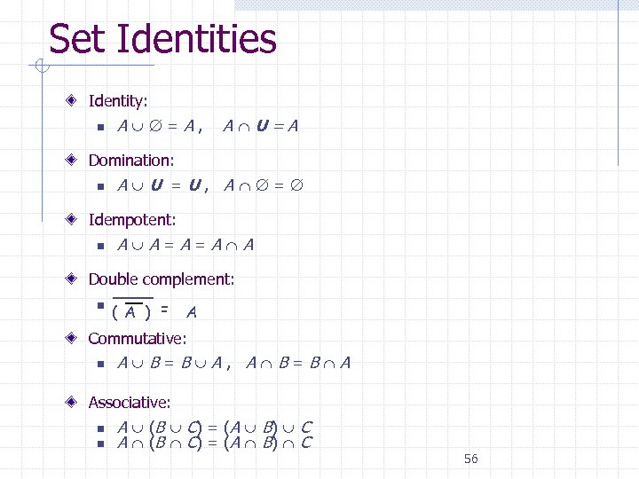Set Identities Identity: n A = A , A U = A Domination: n A U = U , A = Idempotent: n A A = A A Double complement: n ( A ) = A Commutative: n A B = B A , A B = B A Associative: n n A (B C) = (A B) C 56

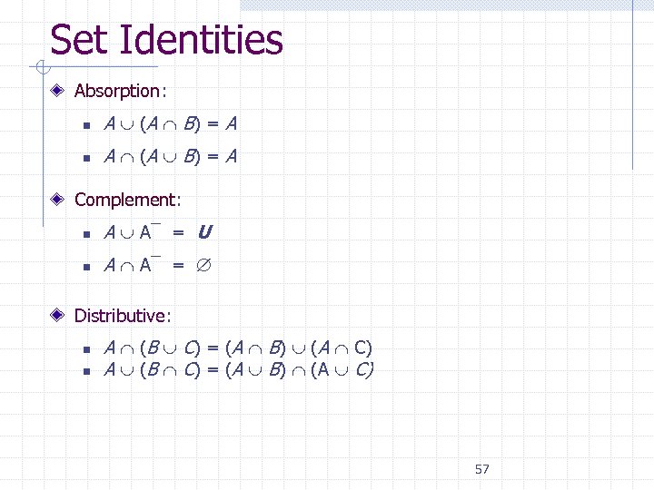Set Identities Absorption: n A (A B) = A Complement: n A A¯ = U n A A¯ = Distributive: n n A (B C) = (A B) (A C) 57

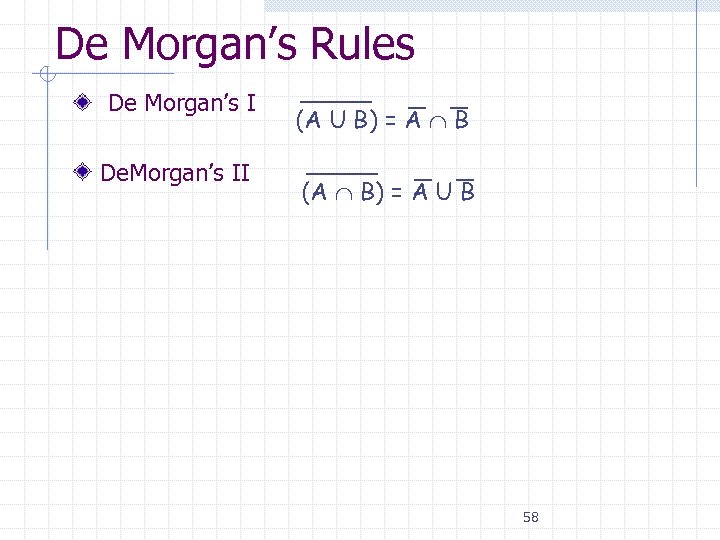De Morgan’s Rules De Morgan’s I De. Morgan’s II (A U B) = A B (A B) = A U B 58

Proving Set Identities How would we prove set identities of the form S 1 = S 2 Where S 1 and S 2 are sets? 1. Prove S 1 S 2 and S 2 S 1 separately. n Use previously proven set identities. n Use logical equivalences to prove equivalent set definitions. 2. Use a membership table. 59

Functions (Section 2. 3) Let A and B be nonempty sets. A function f from A to B is an assignment of exactly one element of B to each element of A. We write f(a) = b if b is the unique element of B assigned by the function f to the element a in A. If f is a function from A to B, we write f : A B. Functions are sometimes called mappings. 60

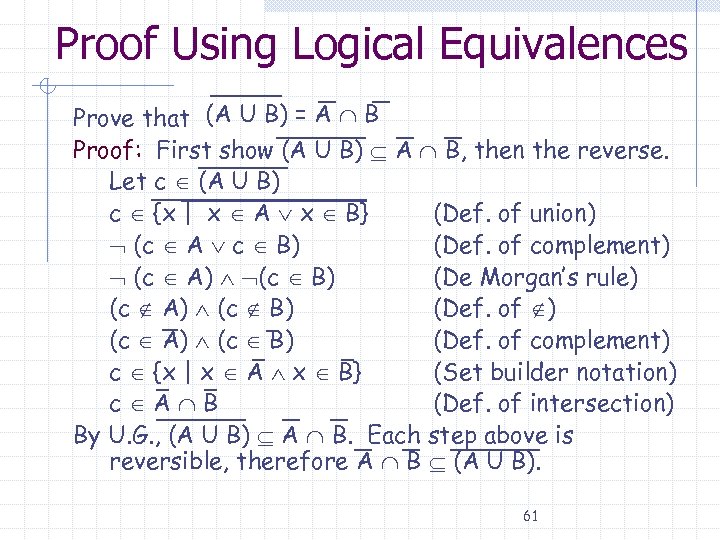Proof Using Logical Equivalences Prove that (A U B) = A B Proof: First show (A U B) A B, then the reverse. Let c (A U B) c {x | x A x B} (Def. of union) (c A c B) (Def. of complement) (c A) (c B) (De Morgan’s rule) (c A) (c B) (Def. of complement) c {x | x A x B} (Set builder notation) c A B (Def. of intersection) By U. G. , (A U B) A B. Each step above is reversible, therefore A B (A U B). 61

Functions (Section 2. 3) Let A and B be nonempty sets. A function f from A to B is an assignment of exactly one element of B to each element of A. We write f(a) = b if b is the unique element of B assigned by the function f to the element a in A. If f is a function from A to B, we write f : A B. Functions are sometimes called mappings. 62

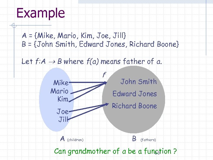Example A = {Mike, Mario, Kim, Joe, Jill} B = {John Smith, Edward Jones, Richard Boone} Let f: A B where f(a) means father of a. Mike Mario Kim Joe Jill A (children) f John Smith Edward Jones Richard Boone B (fathers) Can grandmother of a be a function ? 63

Functions as Ordered Pairs A function f : A B can be represented as a set of ordered pairs (recall, a relation) {(a, b) | a A b = f(a)} A x B For every a A, there is exactly one pair (a, f(a)). 64

Function Terminology Given a function f: A B n A is the domain of f. n B is the codomain of f. n If f(a)=b then b is the image of a under f. n a is the pre-image of b under f. w In general, b may have more than 1 pre-image. n The range R of f (or image of f) is : R = {b | a f(a)=b }. The set of all images of a’s. n For any set S A, the image of S, w f(S) = { b B | a S, f(a) = b} n For any set T B, the inverse image of T w f− 1(T) = { a A | f(a) T } 65

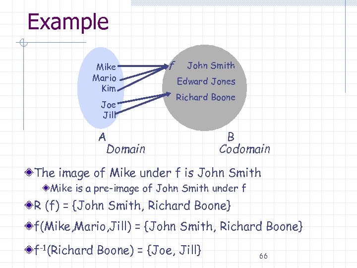Example Mike Mario Kim Joe Jill f John Smith Edward Jones Richard Boone A Domain B Codomain The image of Mike under f is John Smith Mike is a pre-image of John Smith under f R (f) = {John Smith, Richard Boone} f(Mike, Mario, Jill) = {John Smith, Richard Boone} f-1(Richard Boone) = {Joe, Jill} 66

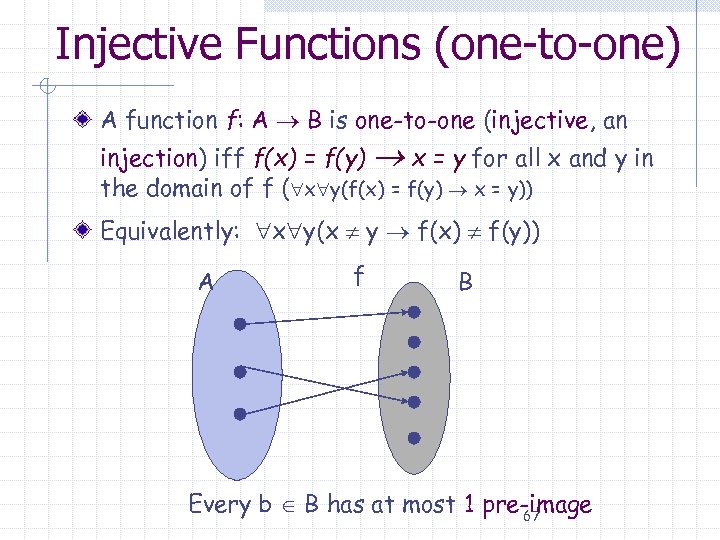Injective Functions (one-to-one) A function f: A B is one-to-one (injective, an injection) iff f(x) = f(y) x = y for all x and y in the domain of f ( x y(f(x) = f(y) x = y)) Equivalently: x y(x y f(x) f(y)) A f B Every b B has at most 1 pre-image 67

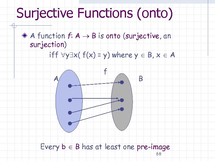Surjective Functions (onto) A function f: A B is onto (surjective, an surjection) iff y x( f(x) = y) where y B, x A A f B Every b B has at least one pre-image 68

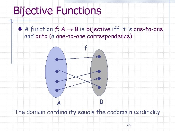Bijective Functions A function f: A B is bijective iff it is one-to-one and onto (a one-to-one correspondence) f B A The domain cardinality equals the codomain cardinality 69

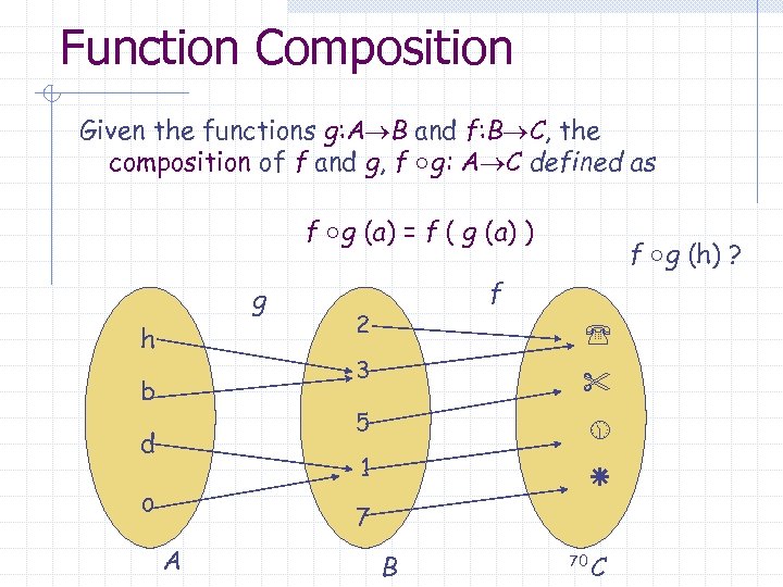Function Composition Given the functions g: A B and f: B C, the composition of f and g, f ○g: A C defined as f ○g (a) = f ( g (a) ) g h f ○g (h) ? f 2 3 o 1 d 5 b 7 A B 70 C

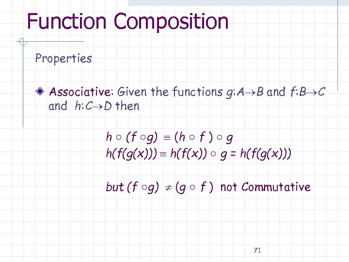Function Composition Properties Associative: Given the functions g: A B and f: B C and h: C D then h ○ (f ○g) (h ○ f ) ○ g h(f(g(x))) h(f(x)) ○ g = h(f(g(x))) but (f ○g) (g ○ f ) not Commutative 71

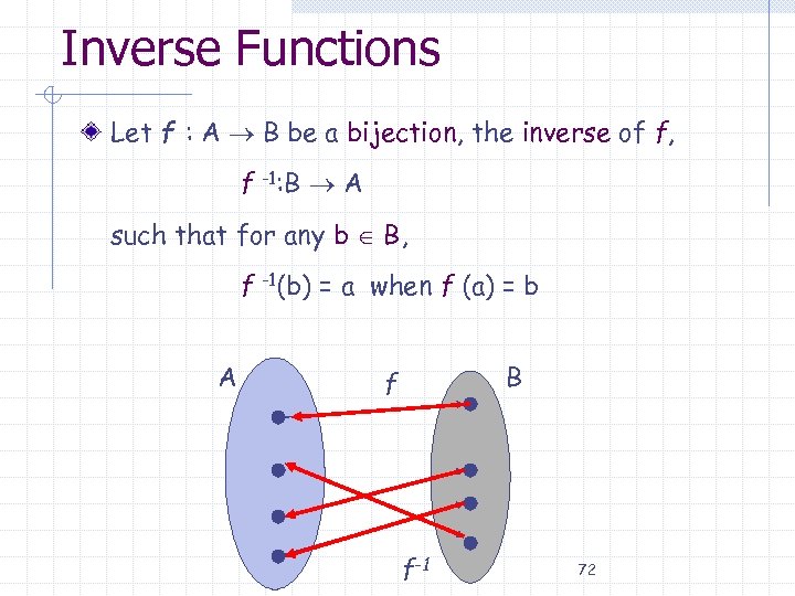Inverse Functions Let f : A B be a bijection, the inverse of f, f -1: B A such that for any b B, f -1(b) = a when f (a) = b A B f f-1 72

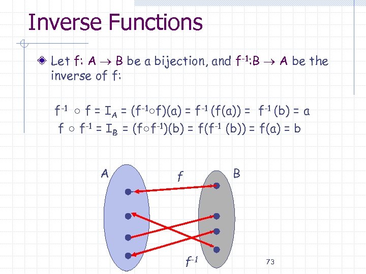Inverse Functions Let f: A B be a bijection, and f-1: B A be the inverse of f: f-1 ○ f = IA = (f-1○f)(a) = f-1 (f(a)) = f-1 (b) = a f ○ f-1 = IB = (f○f-1)(b) = f(f-1 (b)) = f(a) = b A B f f-1 73

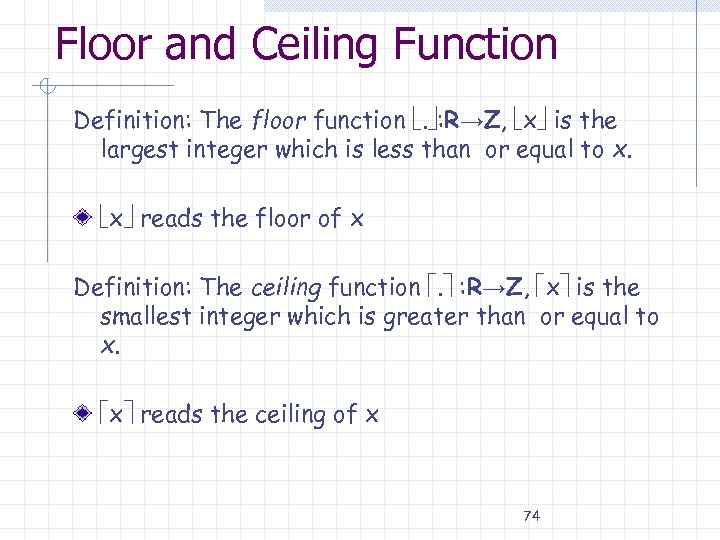Floor and Ceiling Function Definition: The floor function . : R→Z, x is the largest integer which is less than or equal to x. x reads the floor of x Definition: The ceiling function . : R→Z, x is the smallest integer which is greater than or equal to x. x reads the ceiling of x 74

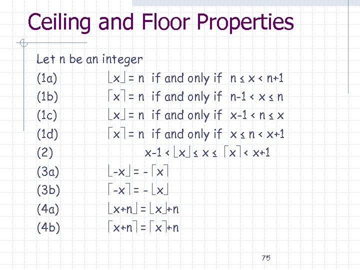Ceiling and Floor Properties Let n be an integer (1 a) x = n if and only if n ≤ x < n+1 (1 b) x = n if and only if n-1 < x ≤ n (1 c) x = n if and only if x-1 < n ≤ x (1 d) x = n if and only if x ≤ n < x+1 (2) x-1 < x ≤ x < x+1 (3 a) -x = - x (3 b) -x = - x (4 a) x+n = x +n (4 b) x+n = x +n 75

Boolean Algebras (Chapter 11) Boolean algebra provides the operations and the rules for working with the set {0, 1}. These are the rules that underlie electronic and optical circuits, and the methods we will discuss are fundamental to VLSI design. 76

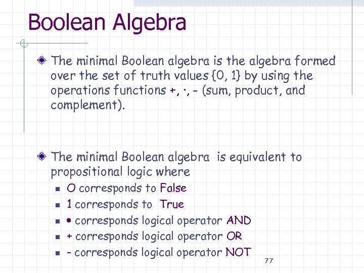Boolean Algebra The minimal Boolean algebra is the algebra formed over the set of truth values {0, 1} by using the operations functions +, ·, - (sum, product, and complement). The minimal Boolean algebra is equivalent to propositional logic where n n n O corresponds to False 1 corresponds to True corresponds logical operator AND + corresponds logical operator OR - corresponds logical operator NOT 77

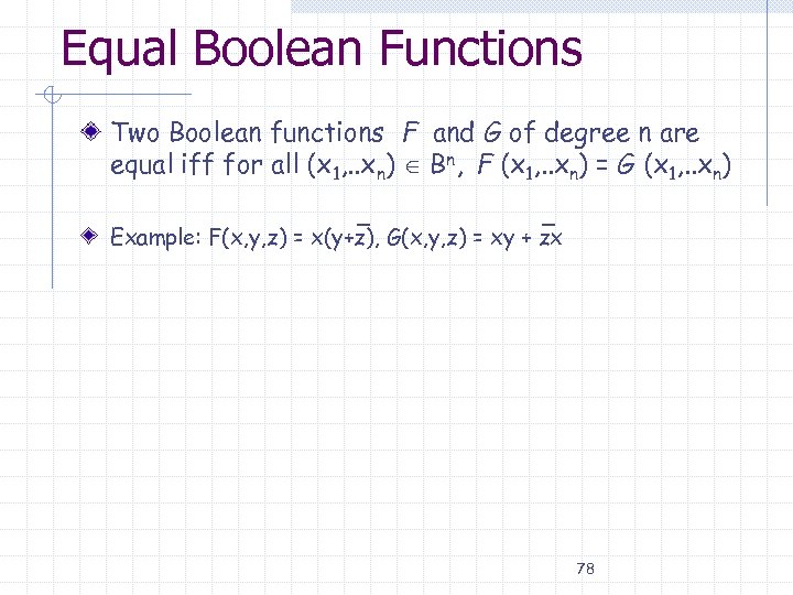Equal Boolean Functions Two Boolean functions F and G of degree n are equal iff for all (x 1, . . xn) Bn, F (x 1, . . xn) = G (x 1, . . xn) Example: F(x, y, z) = x(y+z), G(x, y, z) = xy + zx 78

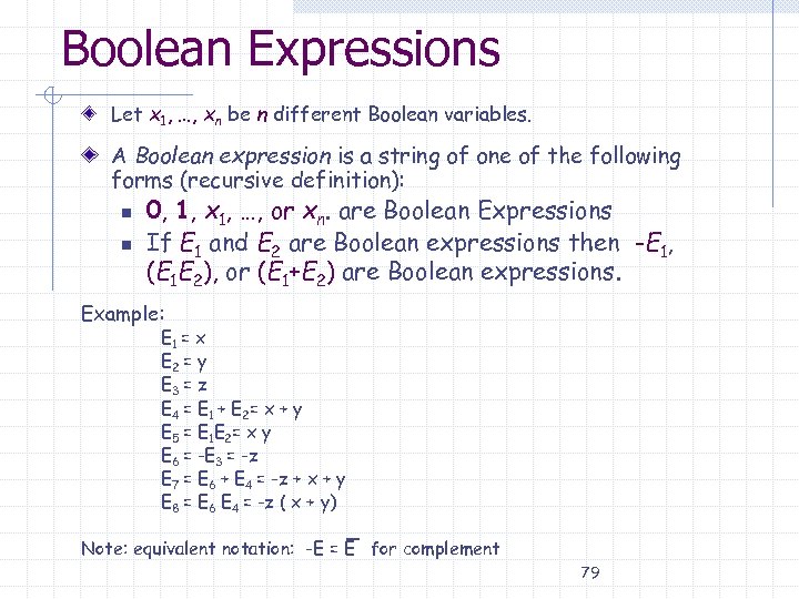Boolean Expressions Let x 1, …, xn be n different Boolean variables. A Boolean expression is a string of one of the following forms (recursive definition): n n 0, 1, x 1, …, or xn. are Boolean Expressions If E 1 and E 2 are Boolean expressions then -E 1, (E 1 E 2), or (E 1+E 2) are Boolean expressions. Example: E 1 = x E 2 = y E 3 = z E 4 = E 1 + E 2 = x + y E 5 = E 1 E 2= x y E 6 = -E 3 = -z E 7 = E 6 + E 4 = -z + x + y E 8 = E 6 E 4 = -z ( x + y) Note: equivalent notation: -E = E for complement 79

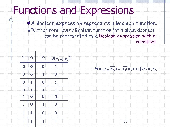Functions and Expressions A Boolean expression represents a Boolean function. n Furthermore, every Boolean function (of a given degree) can be represented by a Boolean expression with n variables. x 1 x 2 x 3 0 0 0 1 0 1 1 0 0 0 1 0 1 1 0 0 1 1 F(x 1, x 2, x 3) = x 1(x 2+x 3)+x 1 x 2 x 3 80

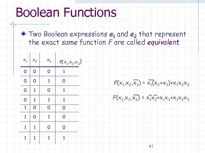Boolean Functions Two Boolean expressions e 1 and e 2 that represent the exact same function F are called equivalent x 1 x 2 x 3 0 0 0 1 0 1 1 0 0 0 1 0 1 1 0 0 1 1 F(x 1, x 2, x 3) = x 1(x 2+x 3)+x 1 x 2 x 3 F(x 1, x 2, x 3) = x 1 x 2+x 1 x 3+x 1 x 2 x 3 81

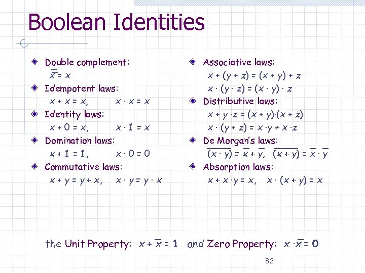Boolean Identities Double complement: x=x Idempotent laws: x + x = x, x·x=x Identity laws: x + 0 = x, x· 1=x Domination laws: x + 1 = 1, x· 0=0 Commutative laws: x + y = y + x, x · y = y · x Associative laws: x + (y + z) = (x + y) + z x · (y · z) = (x · y) · z Distributive laws: x + y ·z = (x + y)·(x + z) x · (y + z) = x ·y + x ·z De Morgan’s laws: (x · y) = x + y, (x + y) = x · y Absorption laws: x + x ·y = x, x · (x + y) = x the Unit Property: x + x = 1 and Zero Property: x ·x = 0 82

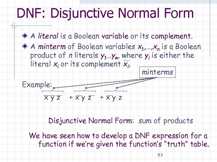DNF: Disjunctive Normal Form A literal is a Boolean variable or its complement. A minterm of Boolean variables x 1, …, xn is a Boolean product of n literals y 1…yn, where yi is either the literal xi or its complement xi. minterms Example: xyz +xyz Disjunctive Normal Form: sum of products We have seen how to develop a DNF expression for a function if we’re given the function’s “truth” table. 83

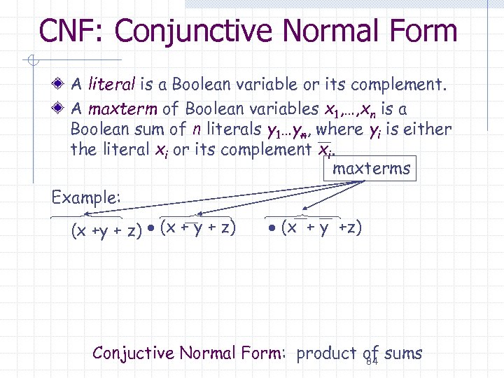CNF: Conjunctive Normal Form A literal is a Boolean variable or its complement. A maxterm of Boolean variables x 1, …, xn is a Boolean sum of n literals y 1…yn, where yi is either the literal xi or its complement xi. maxterms Example: (x +y + z) (x + y +z) Conjuctive Normal Form: product of sums 84

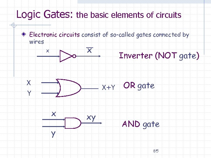Logic Gates: the basic elements of circuits Electronic circuits consist of so-called gates connected by wires x x X Y X+Y x Inverter (NOT gate) y xy OR gate AND gate 85

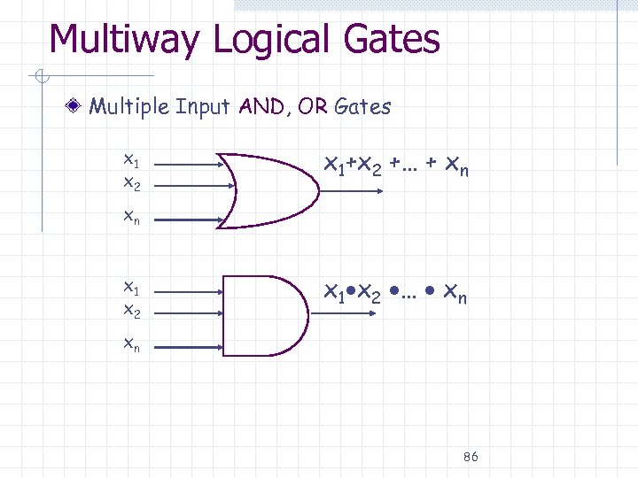Multiway Logical Gates Multiple Input AND, OR Gates x 1 x 2 x 1+x 2 +… + xn xn x 1 x 2 … xn xn 86

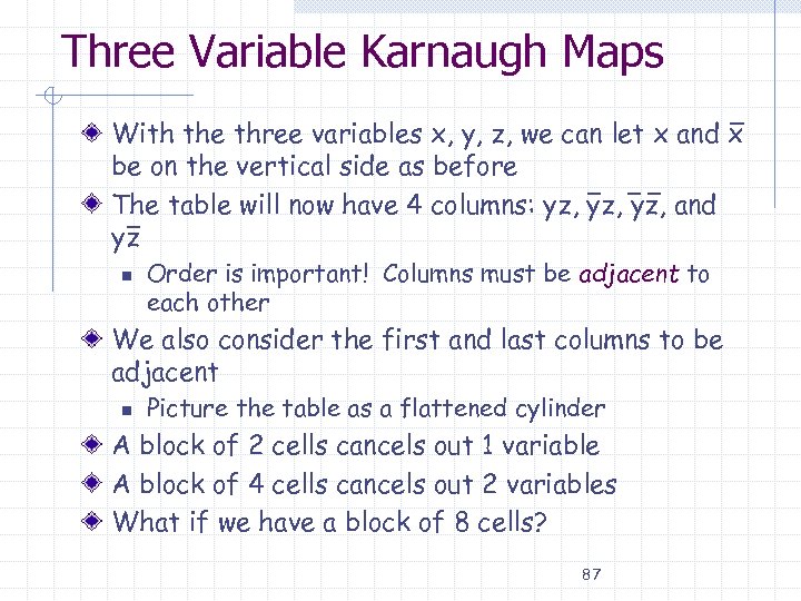Three Variable Karnaugh Maps With the three variables x, y, z, we can let x and x be on the vertical side as before The table will now have 4 columns: yz, yz, and yz n Order is important! Columns must be adjacent to each other We also consider the first and last columns to be adjacent n Picture the table as a flattened cylinder A block of 2 cells cancels out 1 variable A block of 4 cells cancels out 2 variables What if we have a block of 8 cells? 87

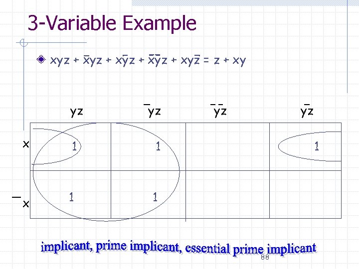3 -Variable Example xyz + xyz = z + xy yz yz x 1 1 yz 1 x yz 1 1 88

Analysis of Algorithms Analyzing an algorithm n n Time complexity Space complexity Time complexity n n Running time needed by an algorithm as a function of the size of the input Denoted as T(N) We are interested in measuring how fast the time complexity increases as the input size grows n Asymptotic Time Complexity of an Algorithm 89

Algorithm Complexity Worst Case Analysis n Largest number of operations to solve a problem of a specified size. n Analyze the worst input case for each input size. n Upper bound of the running time for any input. n Most widely used. Average Case Analysis n Average number of operations over all inputs of a given size w Sometimes it’s too complicated 90

Search Algorithms Search Algorithm Problem: Find an element a in a list a 1, …an (not necessarily ordered) Linear Search Strategy: Examine the sequence one element after another until all the elements have been examined or the current element being examined is the element a. 91

Sorting Algorithms Problem: Given a sequence of numbers, sort the sequence in weakly increasing order. Sorting Algorithms: Input: A sequence of n numbers a 1, a 2, …, an Output: A re-ordering of the input sequence (a’ 1, a’ 2, …, a’n) such that a’ 1 a’ 2 … a’n 92

Sequences (Section 2. 4) Def. : A sequence is a function from a subset of integers I to a set S, (I Z) f: I S Usually, the domain I is either a set of positive or nonnegative consecutive integers {1, 2, 3…} or {0, 1, 2, 3…}. We will usually be using as the domain of I the sequence: I = {i Z | i > 0} Notation: Let i I, the image f(i) is denoted as ai, where ai S ai is called a term of the sequence {ai} represents the entire sequence Note: If the domain I is finite, the sequence is finite, otherwise the sequence is infinite. 93

Sequences Examples: Let the sequence {ai} be defined as ai = i + 3: Terms: a 1, a 2, a 3, … Sequence {ai}: { 4, 5, 6, 7, 8…. } ai = i 2: Terms: a 1, a 2, a 3, … Sequence {ai}: { 1, 4, 9, 16, 25…. } ai = 1/i: Terms: a 1, a 2, a 3, … Sequence {ai}: { 1, 1/2, 1/3, 1/4, 1/5…. } 94

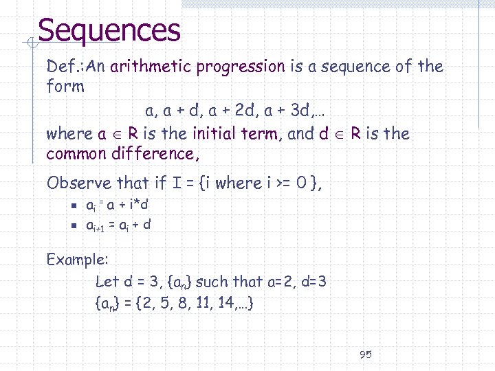Sequences Def. : An arithmetic progression is a sequence of the form a, a + d, a + 2 d, a + 3 d, … where a R is the initial term, and d R is the common difference, Observe that if I = {i where i >= 0 }, n n ai = a + i*d ai+1 = ai + d Example: Let d = 3, {an} such that a=2, d=3 {an} = {2, 5, 8, 11, 14, …} 95

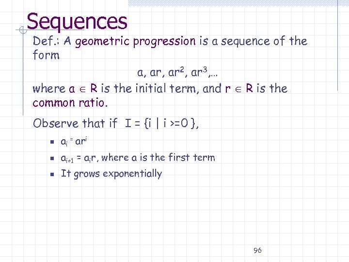Sequences Def. : A geometric progression is a sequence of the form a, ar 2, ar 3, … where a R is the initial term, and r R is the common ratio. Observe that if I = {i | i >=0 }, n ai = ari n ai+1 = air, where a is the first term n It grows exponentially 96

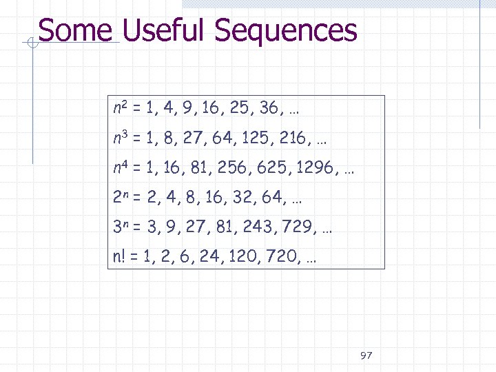Some Useful Sequences n 2 = 1, 4, 9, 16, 25, 36, … n 3 = 1, 8, 27, 64, 125, 216, … n 4 = 1, 16, 81, 256, 625, 1296, … 2 n = 2, 4, 8, 16, 32, 64, … 3 n = 3, 9, 27, 81, 243, 729, … n! = 1, 2, 6, 24, 120, 720, … 97

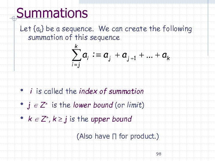Summations Let {ai} be a sequence. We can create the following summation of this sequence h i is called the index of summation h j Z+ is the lower bound (or limit) h k Z+, k j is the upper bound (Also have ∏ for product. ) 98

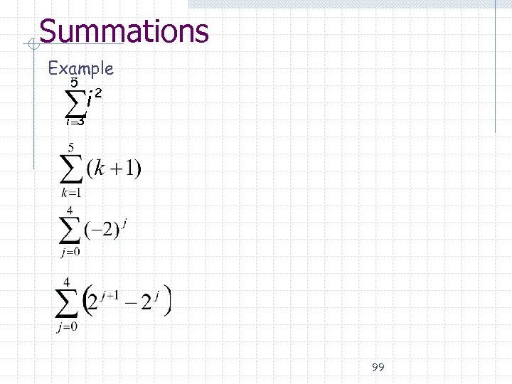Summations Example 5 i 2 i =3 99

Cardinality Def. : The cardinality of a set is the number of elements in the set. Def. : Let A and B be two sets. A and B have the same cardinality iff there is a oneto-one correspondence (bijection) between A and B 100

Countable Sets and Uncountable Sets Def. : Set A is countable if it is finite or if it has the same cardinality as the set of positive integers. Otherwise it is uncountable. (aleph) denotes the cardinality of infinite countable sets Examples: w Infinite Countable Sets: N, Z+, Z-, Z w Infinite Uncountable Sets: R, R+, R- 101

Countable Sets and Uncountable Sets How do you demonstrate that a set is countable ? Suppose A is a set. If there is a one-to-one and onto function f : A Z+, then A is countable. Recall, one-to-one means x y(f(x) = f(y) x = y) onto means y x( f(x) = y) 102

Uncountable sets Theorem: The set of real numbers is uncountable. If a subset of a set is uncountable, then the set is uncountable. The cardinality of a subset is at least as large as the cardinality of the entire set. It is enough to prove that there is a subset of R that is uncountable Theorem: The open interval of real numbers [0, 1) = {r R | 0 r < 1} is uncountable. Proof by contradiction using the Cantor diagonalization argument (Cantor, 1879) 103

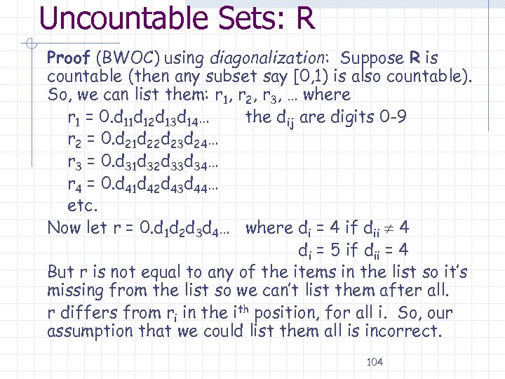Uncountable Sets: R Proof (BWOC) using diagonalization: Suppose R is countable (then any subset say [0, 1) is also countable). So, we can list them: r 1, r 2, r 3, … where r 1 = 0. d 11 d 12 d 13 d 14… the dij are digits 0 -9 r 2 = 0. d 21 d 22 d 23 d 24… r 3 = 0. d 31 d 32 d 33 d 34… r 4 = 0. d 41 d 42 d 43 d 44… etc. Now let r = 0. d 1 d 2 d 3 d 4… where di = 4 if dii 4 d i = 5 if dii = 4 But r is not equal to any of the items in the list so it’s missing from the list so we can’t list them after all. r differs from ri in the ith position, for all i. So, our assumption that we could list them all is incorrect. 104

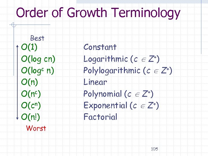Order of Growth Terminology Best O(1) O(log cn) O(logc n) O(nc) O(cn) O(n!) Constant Logarithmic (c Z+) Polylogarithmic (c Z+) Linear Polynomial (c Z+) Exponential (c Z+) Factorial Worst 105

Complexity of Problems Tractable n n n A problem that can be solved with a deterministic polynomial (or better) worst-case time complexity. Also denoted as P Example: w Search Problem w Sorting problem w Find the maximum 106

Complexity of Problems Intractable n Problems that are not tractable. n Example: w Traveling salesperson problem n Wide use of greedy algorithms to get an approximate solution. w For example under certain circumstances you can get an approximation that is at most double the optimal solution. 107

Big-O Notation Big-O notation is used to express the time complexity of an algorithm n n We can assume that any operation requires the same amount of time. The time complexity of an algorithm can be described independently of the software and hardware used to implement the algorithm. 108

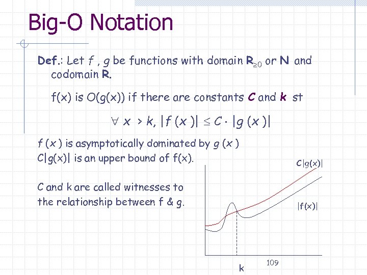Big-O Notation Def. : Let f , g be functions with domain R 0 or N and codomain R. f(x) is O(g(x)) if there are constants C and k st x > k, |f (x )| C |g (x )| f (x ) is asymptotically dominated by g (x ) C|g(x)| is an upper bound of f(x). C|g(x)| C and k are called witnesses to the relationship between f & g. |f(x)| k 109

Big-O Properties Transitivity: if f is O(g) and g is O(h) then f is O(h) Sum Rule: n If f 1 is O(g 1) and f 2 is O(g 2) then f 1+f 2 is O(max(|g 1|, |g 2|)) n If f 1 is O(g) and f 2 is O(g) then f 1+f 2 is O(g) Product Rule n If f 1 is O(g 1) andf 2 is O(g 2) then f 1 f 2 is O(g 1 g 2) For all c > 0, O(cf), O(f + c), O(f c) are O(f) 110

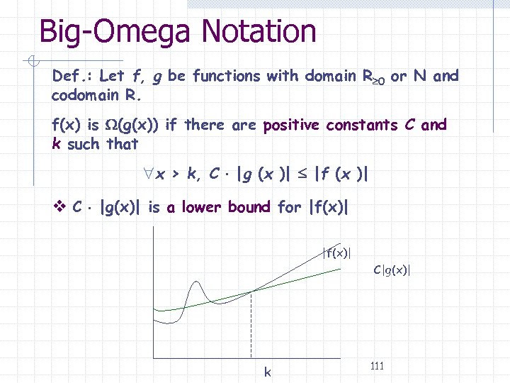Big-Omega Notation Def. : Let f, g be functions with domain R 0 or N and codomain R. f(x) is (g(x)) if there are positive constants C and k such that x > k, C |g (x )| |f (x )| v C |g(x)| is a lower bound for |f(x)| C|g(x)| k 111

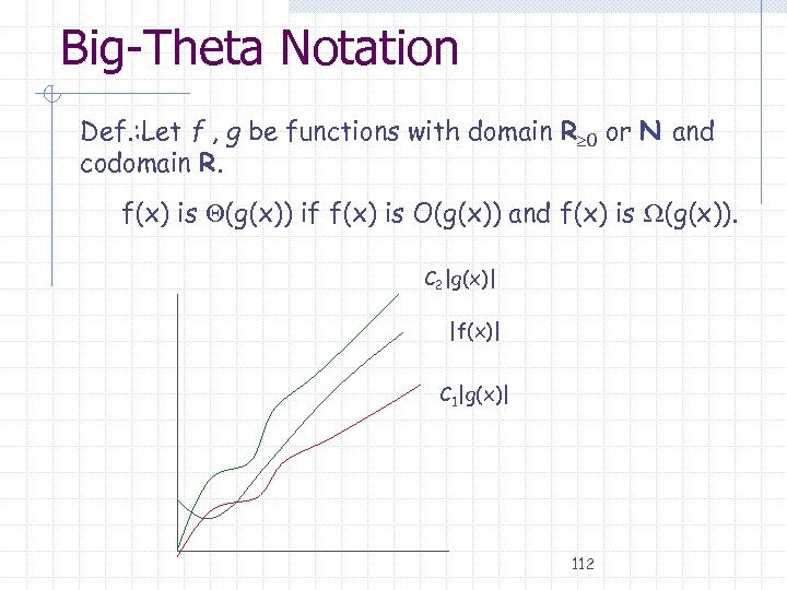Big-Theta Notation Def. : Let f , g be functions with domain R 0 or N and codomain R. f(x) is (g(x)) if f(x) is O(g(x)) and f(x) is (g(x)). C 2|g(x)| |f(x)| C 1|g(x)| 112

Big Summary Upper Bound – Use Big-Oh Lower Bound – Use Big-Omega Upper and Lower (or Order of Growth) – Use Big-Theta 113

Number Theory Elementary number theory, concerned with numbers, usually integers and their properties or rational numbers n n mainly divisibility among integers Modular arithmetic Some Applications n Cryptography w E-commerce w Payment systems w… n n n Random number generation Coding theory Hash functions (as opposed to stew functions ) 114

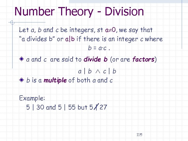Number Theory - Division Let a, b and c be integers, st a 0, we say that “a divides b” or a|b if there is an integer c where b = a·c. a and c are said to divide b (or are factors) a|b c|b b is a multiple of both a and c Example: 5 | 30 and 5 | 55 but 5 | 27 115

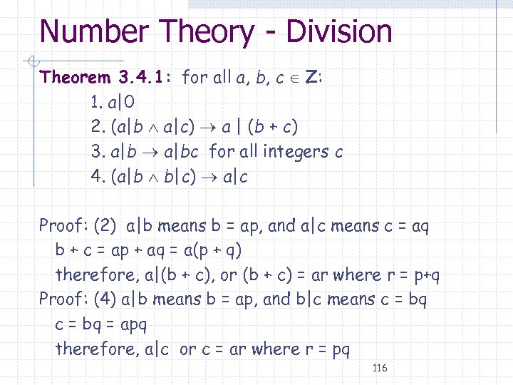Number Theory - Division Theorem 3. 4. 1: for all a, b, c Z: 1. a|0 2. (a|b a|c) a | (b + c) 3. a|bc for all integers c 4. (a|b b|c) a|c Proof: (2) a|b means b = ap, and a|c means c = aq b + c = ap + aq = a(p + q) therefore, a|(b + c), or (b + c) = ar where r = p+q Proof: (4) a|b means b = ap, and b|c means c = bq = apq therefore, a|c or c = ar where r = pq 116

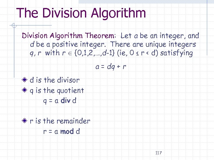The Division Algorithm Theorem: Let a be an integer, and d be a positive integer. There are unique integers q, r with r {0, 1, 2, …, d-1} (ie, 0 ≤ r < d) satisfying a = dq + r d is the divisor q is the quotient q = a div d r is the remainder r = a mod d 117

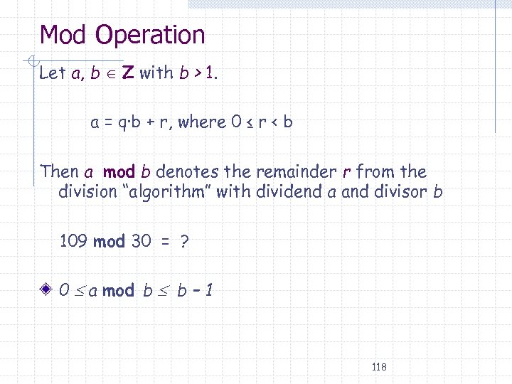Mod Operation Let a, b Z with b > 1. a = q·b + r, where 0 ≤ r < b Then a mod b denotes the remainder r from the division “algorithm” with dividend a and divisor b 109 mod 30 = ? 0 a mod b b – 1 118

Modular Arithmetic Let a, b Z, m Z+ Then a is congruent to b modulo m iff m | (a b). Notation: n n “a b (mod m)” reads a is congruent to b modulo m “a b (mod m)” reads a is not congruent to b modulo m. Examples: n n 5 25 (mod 10) 5 25 (mod 3) 119

Modular Arithmetic Theorem 3. 4. 3: Let a, b Z, m Z+. Then a b (mod m) iff a mod m = b mod m Proof: (1) given a mod m = b mod m we have a = ms + r or r = a – ms, b = mp + r or r = b – mp, a – ms = b – mp which means a – b = ms – mp = m(s – p) so m | (a – b) which means a b (mod m) 120

Modular Arithmetic Theorem 3. 4. 3: Let a, b Z, m Z+. Then a b (mod m) iff a mod m = b mod m Proof: (2) given a b (mod m) we have m | (a – b) let a = mqa + ra and b = mqb + rb so, m|((mqa + ra) – (mqb + rb)) or m|m(qa – qb) + (ra – rb) recall 0 ≤ ra < m and 0 ≤ rb < m therefore (ra – rb) must be 0 that is, the two remainders are the same which is the same as saying a mod m = b mod m 121

Modular Arithmetic Theorem 3. 4. 4: Let a, b Z, m Z+. Then: a b (mod m) iff there exists a k Z st a = b + km. Proof: a = b + km means a – b = km which means m | (a – b) which is the same as saying a b (mod m) (to complete the proof, reverse the steps) Examples: 27 12 (mod 5) 27 = 12 + 5 k k=3 105 -45 (mod 10) 105 = -45 + 10 k k = 15 122

Modular Arithmetic Theorem 3. 4. 5: Let a, b, c, d Z, m Z+. Then if a b (mod m) and c d (mod m), then: 1. a + c b + d (mod m), 2. a - c b - d (mod m), 3. ac bd (mod m) Proof: a = b + k 1 m and c = d + k 2 m a + c = b + d + k 1 m + k 2 m or a + c = b + d + m(k 1 + k 2) which is a + c b + d (mod m) others are similar 123

Number Theory - Primes A positive integer n > 1 is called prime if it is only divisible by 1 and itself (i. e. , only has 1 and itself as its positive factors). Example: 2, 3, 5, 7, 11, 13, 17, 19, 23, 29, 31, 97 A number n 2 which isn’t prime is called composite. Example: All even numbers > 2 are composite. By convention, 1 is neither prime or composite. 124

Number Theory - Primes Fundamental Theorem of Arithmetic Every positive integer greater than 1 has a unique representation as the product of a non-decreasing series of one or more primes Examples: w w w 2=2 4 = 2· 2 100 = 2· 2· 5· 5 200 = 2· 2· 2· 5· 5 999= 3· 3· 3· 37 125

Number Theory – Prime Numbers Theorem 3. 5. 3: There are infinitely many primes. We proved earlier in the semester that for any integer x, there exists a prime number p such that p > x. Let (n) = | {p | p ≤ n and p is prime} | 126

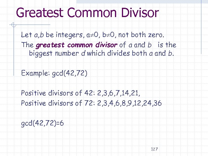Greatest Common Divisor Let a, b be integers, a 0, b 0, not both zero. The greatest common divisor of a and b is the biggest number d which divides both a and b. Example: gcd(42, 72) Positive divisors of 42: 2, 3, 6, 7, 14, 21, Positive divisors of 72: 2, 3, 4, 6, 8, 9, 12, 24, 36 gcd(42, 72)=6 127

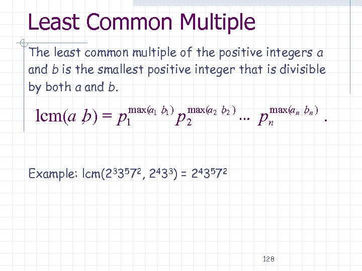Least Common Multiple The least common multiple of the positive integers a and b is the smallest positive integer that is divisible by both a and b. max( = p 1 max(a 1 , b 1 ) p 2 a 2 , b 2 ) … pn an , bn ). lcm(a , b) Example: lcm(233572, 2433) = 243572 128

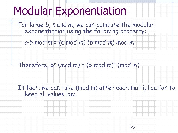Modular Exponentiation For large b, n and m, we can compute the modular exponentiation using the following property: a·b mod m = (a mod m) (b mod m) mod m Therefore, bn (mod m) = (b mod m)n (mod m) In fact, we can take (mod m) after each multiplication to keep all values low. 129

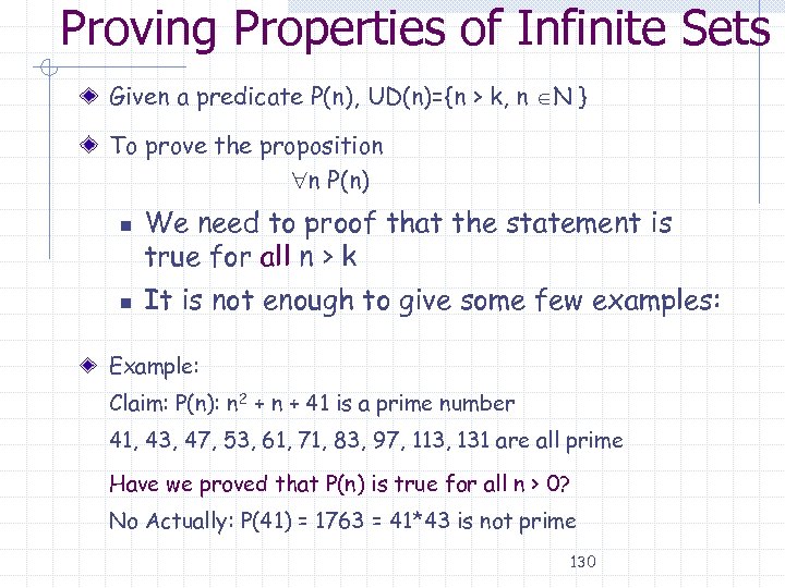Proving Properties of Infinite Sets Given a predicate P(n), UD(n)={n > k, n N } To prove the proposition n P(n) n n We need to proof that the statement is true for all n > k It is not enough to give some few examples: Example: Claim: P(n): n 2 + n + 41 is a prime number 41, 43, 47, 53, 61, 71, 83, 97, 113, 131 are all prime Have we proved that P(n) is true for all n > 0? No Actually: P(41) = 1763 = 41*43 is not prime 130

Weak Mathematical Induction Principle of Weak Mathematical Induction 1) [Base Case] P (m) is true for some m N Usually (but not always) the base case is proved for m = 0 or 1 2) [Inductive Step] Inductive Hypothesis: Assume that P(n) is true, for an arbitrary n such that n ≥ m Prove 3) Then: P(n) P(n+1) n ≥ m P(n) is true Idea: If it’s true for n=1, then it’s true for n=2. If it’s true for n=2, then it’s true for n=3. If it’s true for n=3, then it’s true for n = 4 … [P (m) n m (P (n) P(n + 1))] n m P (n) 131

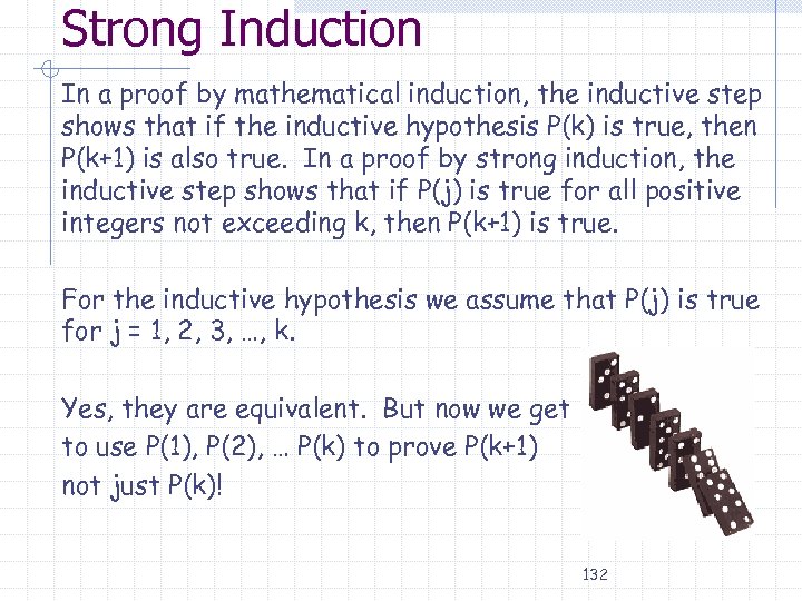Strong Induction In a proof by mathematical induction, the inductive step shows that if the inductive hypothesis P(k) is true, then P(k+1) is also true. In a proof by strong induction, the inductive step shows that if P(j) is true for all positive integers not exceeding k, then P(k+1) is true. For the inductive hypothesis we assume that P(j) is true for j = 1, 2, 3, …, k. Yes, they are equivalent. But now we get to use P(1), P(2), … P(k) to prove P(k+1) not just P(k)! 132

Strong Induction Principle of Strong Induction 1) [Base Case] show P (1) is true 2) [Inductive Step] assume P(j) for j = 1, 2, …, k Inductive Hypothesis: Prove P(1) P(2) … P(k) P(k+1) 133

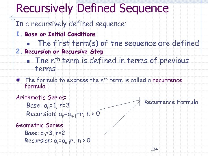Recursively Defined Sequence In a recursively defined sequence: 1. Base or Initial Conditions n The first term(s) of the sequence are defined 2. Recursion or Recursive Step n The nth term is defined in terms of previous terms The formula to express the nth term is called a recurrence formula Arithmetic Series: Base: a 0=1, r=3 Recursion: an=an-1+r, n > 0 Recurrence Formula Geometric Series Base: a 0=3, r=2 Recursion: an=an-1 r, n > 0 134

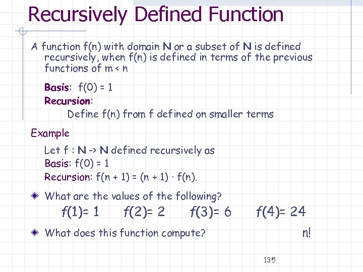Recursively Defined Function A function f(n) with domain N or a subset of N is defined recursively, when f(n) is defined in terms of the previous functions of m < n Basis: f(0) = 1 Recursion: Define f(n) from f defined on smaller terms Example Let f : N -> N defined recursively as Basis: f(0) = 1 Recursion: f(n + 1) = (n + 1) · f(n). What are the values of the following? f(1)= 1 f(2)= 2 f(3)= 6 f(4)= 24 n! What does this function compute? 135

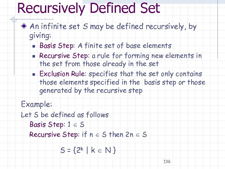Recursively Defined Set An infinite set S may be defined recursively, by giving: n n n Basis Step: A finite set of base elements Recursive Step: a rule forming new elements in the set from those already in the set Exclusion Rule: specifies that the set only contains those elements specified in the basis step or those generated by the recursive step Example: Let S be defined as follows Basis Step: 1 S Recursive Step: if n S then 2 n S S = {2 k | k N } 136

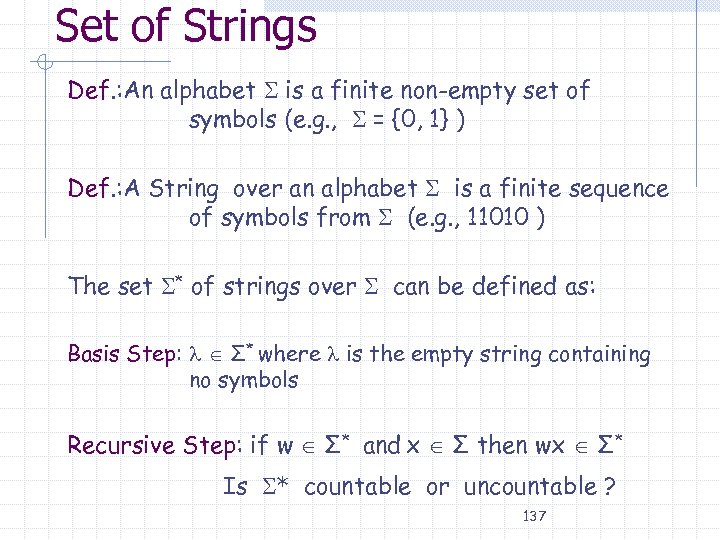Set of Strings Def. : An alphabet is a finite non-empty set of symbols (e. g. , = {0, 1} ) Def. : A String over an alphabet is a finite sequence of symbols from (e. g. , 11010 ) The set * of strings over can be defined as: Basis Step: Σ* where is the empty string containing no symbols Recursive Step: if w Σ* and x Σ then wx Σ* Is * countable or uncountable ? 137

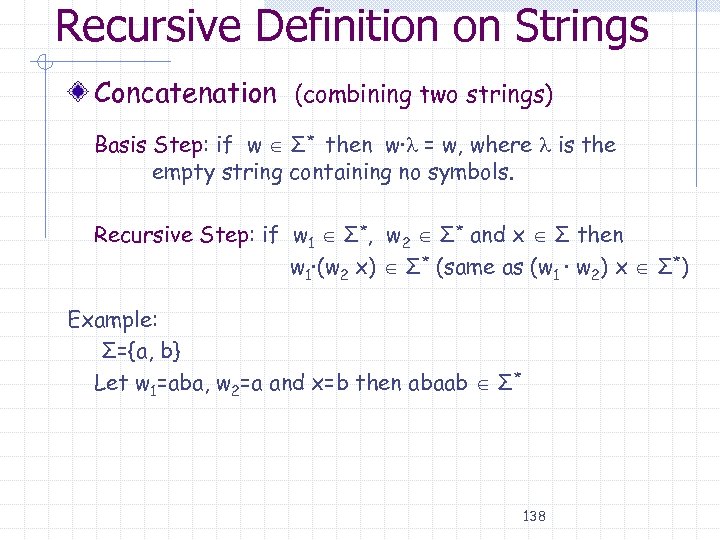Recursive Definition on Strings Concatenation (combining two strings) Basis Step: if w Σ* then w· = w, where is the empty string containing no symbols. Recursive Step: if w 1 Σ*, w 2 Σ* and x Σ then w 1·(w 2 x) Σ* (same as (w 1 · w 2) x Σ*) Example: Σ={a, b} Let w 1=aba, w 2=a and x=b then abaab Σ* 138

Counting (now in chapter 5) The basic counting principles are the product rule and sum rule. Product Rule: Suppose that a procedure can be broken down into a sequence of two tasks. If there are n ways to do the first task and for each of these ways of doing the first task, there are m ways to do the second task, then there are n·m ways to do the procedure. Sum Rule: If a task can be done either in one of n ways or in one of m ways, where none of the set of n ways is the same as any of the set of m ways, then there are n + m ways to do the task. 139

Counting The Pigeonhole Principle: If k is a positive integer and k+1 or more objects are placed in k boxes, then there is at least one box containing two or more of the objects. (prove BWOC) Of 367 people, at least two have the same birth day. For every integer n there is a multiple of n that has only 0 s and 1 s in its decimal expansion. 140

Counting Part of combinatorics, the study of arrangements of objects. (Sets, sequences, sebsets, etc. ) Counting relies on two important, but simple principles: the Product Rule and Sum Rule 141

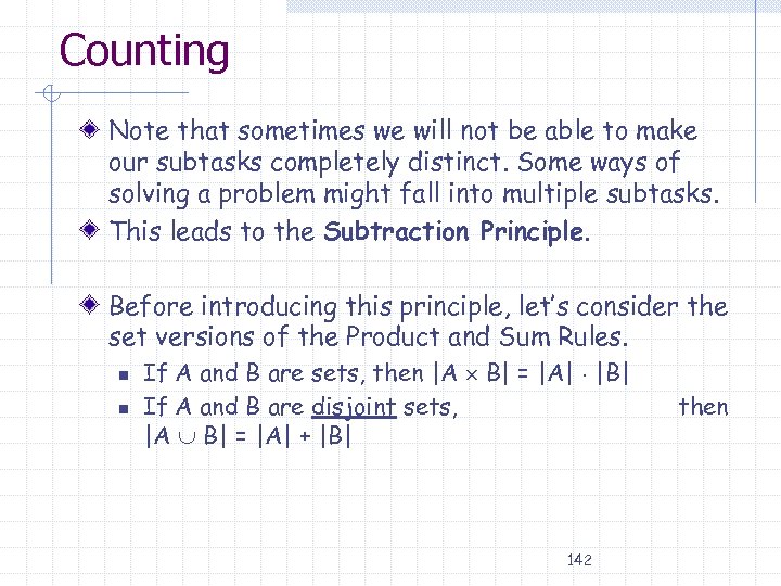Counting Note that sometimes we will not be able to make our subtasks completely distinct. Some ways of solving a problem might fall into multiple subtasks. This leads to the Subtraction Principle. Before introducing this principle, let’s consider the set versions of the Product and Sum Rules. n n If A and B are sets, then |A B| = |A| |B| If A and B are disjoint sets, |A B| = |A| + |B| 142 then

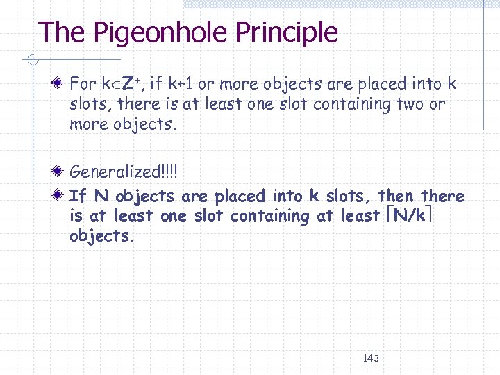The Pigeonhole Principle For k Z+, if k+1 or more objects are placed into k slots, there is at least one slot containing two or more objects. Generalized!!!! If N objects are placed into k slots, then there is at least one slot containing at least N/k objects. 143

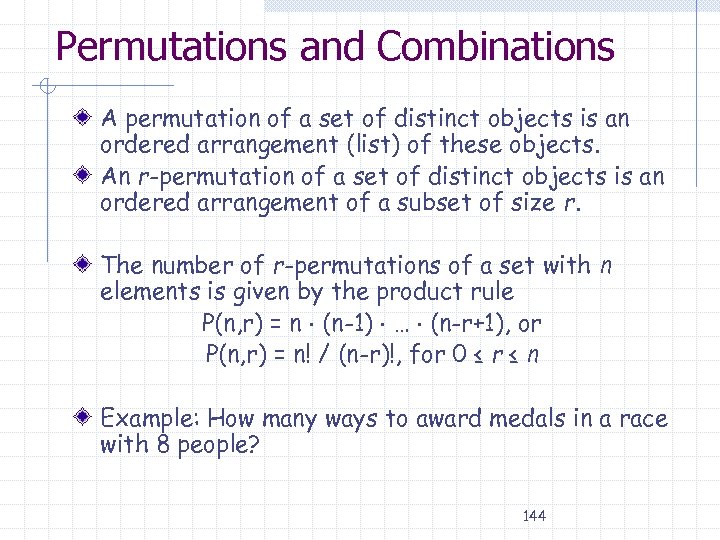Permutations and Combinations A permutation of a set of distinct objects is an ordered arrangement (list) of these objects. An r-permutation of a set of distinct objects is an ordered arrangement of a subset of size r. The number of r-permutations of a set with n elements is given by the product rule P(n, r) = n (n-1) … (n-r+1), or P(n, r) = n! / (n-r)!, for 0 ≤ r ≤ n Example: How many ways to award medals in a race with 8 people? 144

Permutations and Combinations An r-combination of a set of distinct objects is an unordered arrangement (subset) of size r. The number of r-combinations of a set with n elements is given by C(n, r) = n! / [r! (n-r)!], for 0 ≤ r ≤ n The binomial coefficient symbolism is also used. (More on that later!) Examples: n n How many 5 card poker hands are there? How many bitstrings of length six contain exactly three 0’s? 145

Probability We can understand probability by considering sets of outcomes: We define a set S to be a sample space, a set of all possible outcomes of some experiment. We define a set E S, the set of all outcomes in which the event occurs. We further assume that all outcomes in S are equally likely. Then the probability of the event occurring is: p(E) = |E| / |S| 146

Probability We use p(E) to denote the probability that an event occurs. We use p(E) to denote the probability that an event does not occur. P(E) = 1 – p(E) If a coin is flipped 5 times, what is the probability of at least one head coming up? 147

Probability If E 1 and E 2 are two events in the sample space, then p(E 1 E 2) = p(E 1) + p(E 2) – p(E 1 E 2) It’s just the subtraction principle again! A number is selected at random from the set of positive integers less than or equal to 100. What is the probability the number is divisible by either 2 or 5? 148

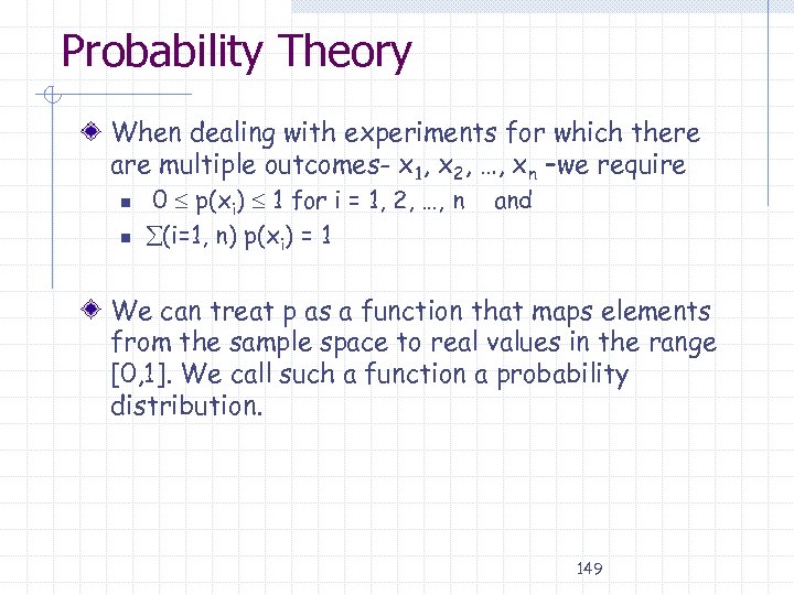Probability Theory When dealing with experiments for which there are multiple outcomes- x 1, x 2, …, xn –we require n n 0 p(xi) 1 for i = 1, 2, …, n (i=1, n) p(xi) = 1 and We can treat p as a function that maps elements from the sample space to real values in the range [0, 1]. We call such a function a probability distribution. 149

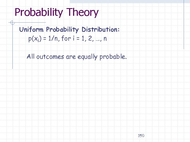Probability Theory Uniform Probability Distribution: p(xi) = 1/n, for i = 1, 2, …, n All outcomes are equally probable. 150

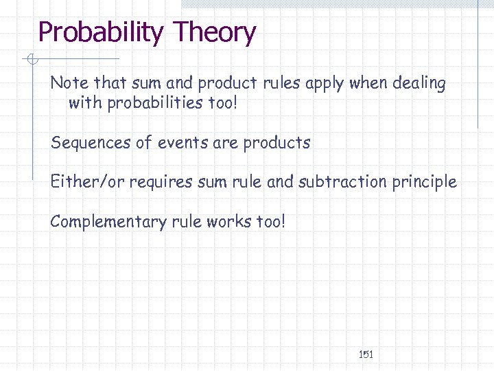Probability Theory Note that sum and product rules apply when dealing with probabilities too! Sequences of events are products Either/or requires sum rule and subtraction principle Complementary rule works too! 151

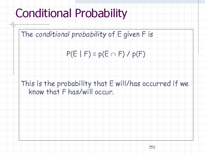Conditional Probability The conditional probability of E given F is P(E | F) = p(E F) / p(F) This is the probability that E will/has occurred if we know that F has/will occur. 152

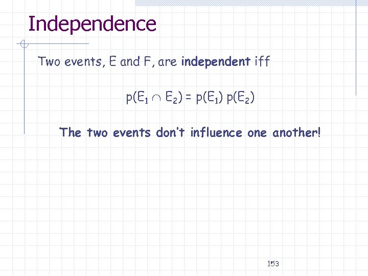Independence Two events, E and F, are independent iff p(E 1 E 2) = p(E 1) p(E 2) The two events don’t influence one another! 153

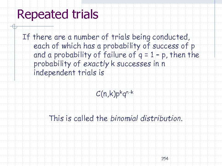Repeated trials If there a number of trials being conducted, each of which has a probability of success of p and a probability of failure of q = 1 – p, then the probability of exactly k successes in n independent trials is C(n, k)pkqn-k This is called the binomial distribution. 154

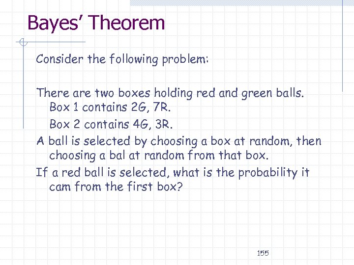Bayes’ Theorem Consider the following problem: There are two boxes holding red and green balls. Box 1 contains 2 G, 7 R. Box 2 contains 4 G, 3 R. A ball is selected by choosing a box at random, then choosing a bal at random from that box. If a red ball is selected, what is the probability it cam from the first box? 155

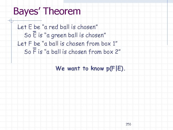Bayes’ Theorem Let E be “a red ball is chosen” So E is “a green ball is chosen” Let F be “a ball is chosen from box 1” So F is “a ball is chosen from box 2” We want to know p(F|E). 156

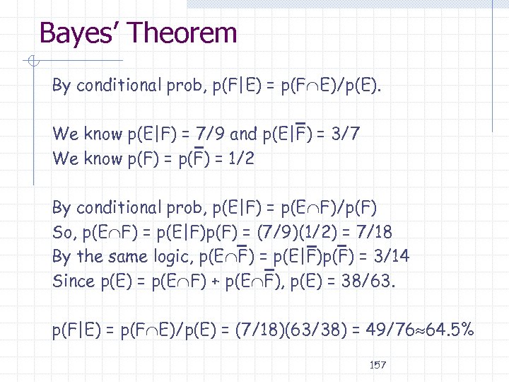Bayes’ Theorem By conditional prob, p(F|E) = p(F E)/p(E). We know p(E|F) = 7/9 and p(E|F) = 3/7 We know p(F) = 1/2 By conditional prob, p(E|F) = p(E F)/p(F) So, p(E F) = p(E|F)p(F) = (7/9)(1/2) = 7/18 By the same logic, p(E F) = p(E|F)p(F) = 3/14 Since p(E) = p(E F) + p(E F), p(E) = 38/63. p(F|E) = p(F E)/p(E) = (7/18)(63/38) = 49/76 64. 5% 157

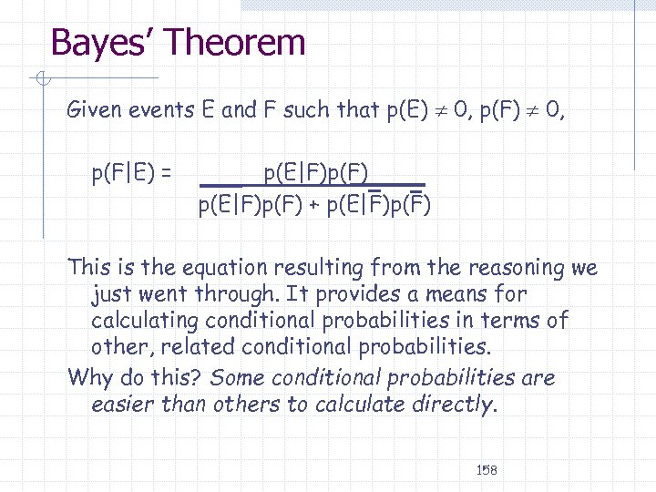Bayes’ Theorem Given events E and F such that p(E) 0, p(F|E) = p(E|F)p(F) + p(E|F)p(F) This is the equation resulting from the reasoning we just went through. It provides a means for calculating conditional probabilities in terms of other, related conditional probabilities. Why do this? Some conditional probabilities are easier than others to calculate directly. 158

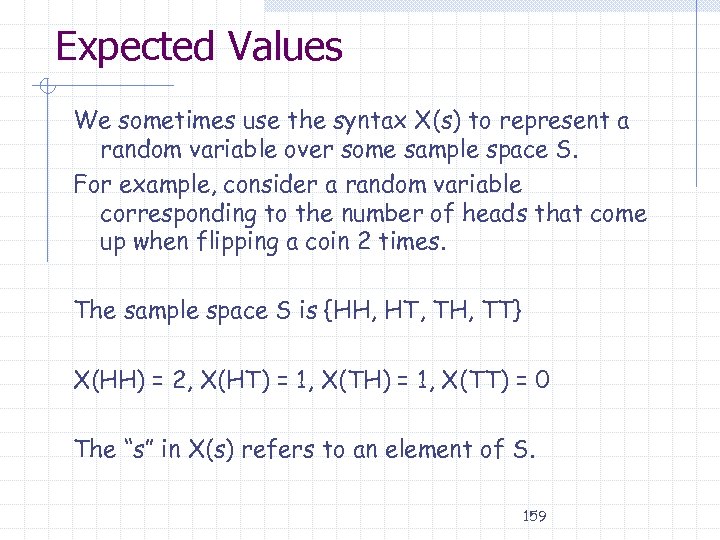Expected Values We sometimes use the syntax X(s) to represent a random variable over some sample space S. For example, consider a random variable corresponding to the number of heads that come up when flipping a coin 2 times. The sample space S is {HH, HT, TH, TT} X(HH) = 2, X(HT) = 1, X(TH) = 1, X(TT) = 0 The “s” in X(s) refers to an element of S. 159

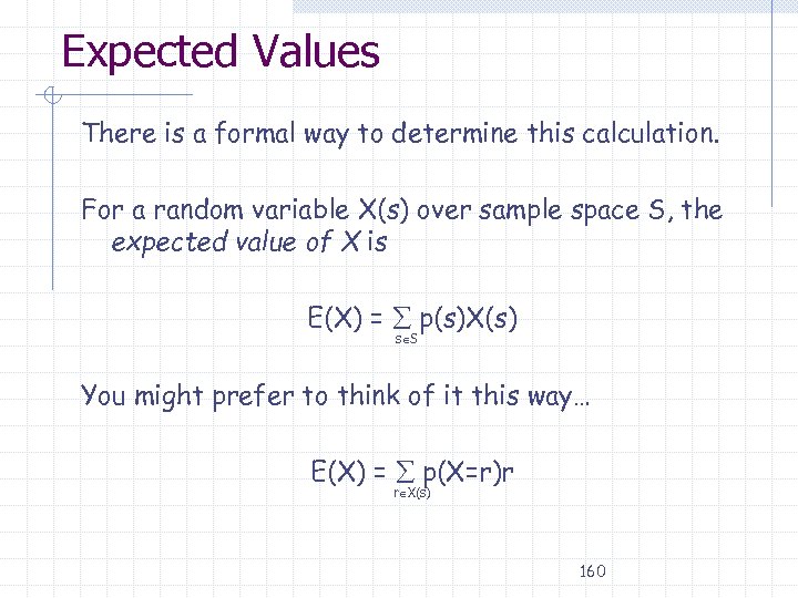Expected Values There is a formal way to determine this calculation. For a random variable X(s) over sample space S, the expected value of X is E(X) = p(s)X(s) s S You might prefer to think of it this way… E(X) = p(X=r)r r X(s) 160

Variance Expected value gives us an important piece of information regarding a distribution or random variable. It’s like knowing the average grade for the class. But the class average doesn’t tell us how spread out the classes scores were. For that we need another measure- a measure of spread. 161

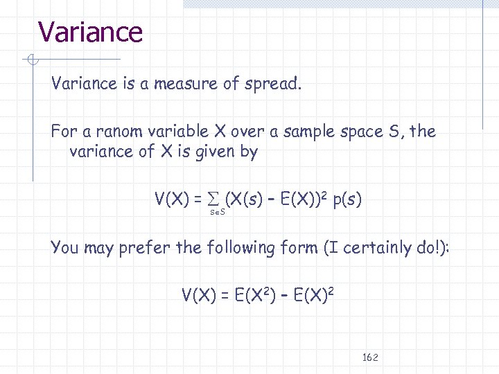Variance is a measure of spread. For a ranom variable X over a sample space S, the variance of X is given by V(X) = (X(s) – E(X))2 p(s) s S You may prefer the following form (I certainly do!): V(X) = E(X 2) – E(X)2 162

Standard Deviation Combined, variance and expected value can give a lot of information. Many distributions, such as the Normal distribution (bell curve), are defined in terms of these two parameters. The standard deviation of X is sometimes used instead of variance. It has nice properties that you may learn about if you take a course in probability of statistics. The standard deviation of X is given by (X) = V(X)½ 163

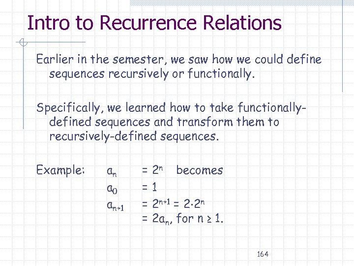Intro to Recurrence Relations Earlier in the semester, we saw how we could define sequences recursively or functionally. Specifically, we learned how to take functionallydefined sequences and transform them to recursively-defined sequences. Example: an a 0 an+1 = 2 n becomes =1 = 2 n+1 = 2 2 n = 2 an, for n ≥ 1. 164

Intro to Recurrence Relations Solving recurrence relations works in the opposite direction. But there’s a catch… (Isn’t there always? ) A recursive definition of a sequence involves a recursive formula and a set of basis values. The formula itself, without the initial conditions, is a recurrence relation. We are going to be interested in solving relations both with, and without, initial conditions. 165

Intro to Recurrence Relations Without initial conditions, a recurrence relation defines a set, or family, of sequences. Consider an+1 = 2 an. If a 0 = 1, an = 2 n. But if a 0 = 3, an = 3 2 n. These two sequences are clearly similar. This is because an+1 = 2 an defines a family of sequences, an = a 0 2 n, for n ≥ 1. 166

Intro to Recurrence Relations A recurrence relation along with initial conditions specify a single sequence. Any such sequence is a solution to the relation. We can check solutions using substitution. Consider the recurrence relation an = 2 an-1 - an-2. Is an = 3 n a solution for n ≥ 1? Try it out! an = 2 an-1 - an-2 = 2 3(n-1) – 3(n-2) = 6 n – 6 -3 n + 6 = 3 n = an 167

Intro to Recurrence Relations Finally, let’s see how we can apply recurrence relations and their solutions to a tough counting problem. How many bitstrings of length n do not contain consecutive 0’s? The techniques we’ve studied so far can’t solve this without ridiculous amounts of effort! One solution is 5 -½( (1+5½)/2 )n+2 - 5 -½( (1 -5½)/2 )n+2. We can find a more elegant and easier solution!!! 168