efe781f130bb9e0c1319723e6b792430.ppt
- Количество слайдов: 48
 Discrete choice models Chapter 16 Statistics for Marketing & Consumer Research Copyright © 2008 - Mario Mazzocchi 1
 Choice models and preferences • Choice modeling is the preferred model for studies on consumer preferences • Choice models are closely related stated preference theory • Stated preference survey: consumers state their choices among a potential set of alternatives (e. g. different brands, different product characteristics, different stores) • Options can include both real and hypothetical market alternatives • Choice models start from stated preferences to go back to their determinants • The alternative to stated preference is revealed preference • where consumers are not asked directly what they prefer or choose but their actual choices and determinants are observed indirectly, for example considering what they purchase in different situations Statistics for Marketing & Consumer Research Copyright © 2008 - Mario Mazzocchi 2
 Stated vs. revealed preference • Example • A customer finds that the price of her favourite washing powder in her usual supermarket has doubled • Will she buy less washing powder, like a smaller pack? • Or would she move to a different brand? • Would she go back home without buying washing powder at all? • It could be difficult to define a model which explains choices using revealed preference, i. e. observing behaviors at the checkout till – if the customer decides not to buy washing powder at all, how would it be possible to infer this choice simply from a look at the products in her shopping trolley? – if the customer buys an alternative brand with exactly the same size and price as before the price increase would a revealed preference model capture that consumer decision? Statistics for Marketing & Consumer Research Copyright © 2008 - Mario Mazzocchi 3
 Stated vs. revealed preference • Revealed preference allows one to model these behaviors, but only after an expensive collection of information on the frequency quantity and brands of washing powder purchases • Stated preference alternative • a survey where the consumer is asked to choose between a set of alternative choices which differ by brand, pack size and price • Provided that the survey is designed in an appropriate way (not necessarily easy) the collected data open the way to a more effective model Statistics for Marketing & Consumer Research Copyright © 2008 - Mario Mazzocchi 4
 Choice models • Consumer models are usually targeted on the average behaviour • With revealed preference one might apply a regression model; where we purchased the quantity is the dependent variable and price and other explanatory variables are on the right-hand side. • With stated preference models a discrete choice variable is on the left-hand side of the equation • • • Example the choice whether to purchase washing powder or not (binary dependent variable); choice among a set of alternative brands (categorical DV) Statistics for Marketing & Consumer Research Copyright © 2008 - Mario Mazzocchi 5
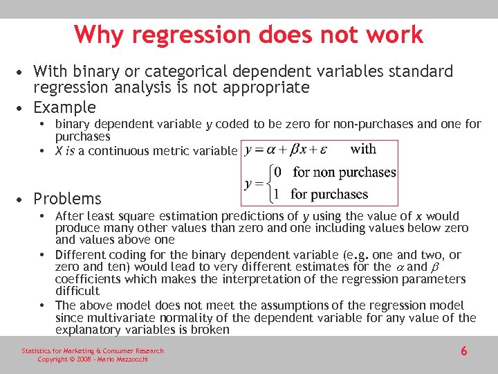 Why regression does not work • With binary or categorical dependent variables standard regression analysis is not appropriate • Example • binary dependent variable y coded to be zero for non-purchases and one for purchases • X is a continuous metric variable • Problems • After least square estimation predictions of y using the value of x would produce many other values than zero and one including values below zero and values above one • Different coding for the binary dependent variable (e. g. one and two, or zero and ten) would lead to very different estimates for the a and b coefficients which makes the interpretation of the regression parameters difficult • The above model does not meet the assumptions of the regression model since multivariate normality of the dependent variable for any value of the explanatory variables is broken Statistics for Marketing & Consumer Research Copyright © 2008 - Mario Mazzocchi 6
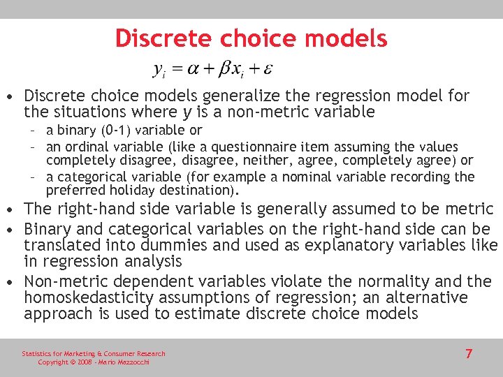 Discrete choice models • Discrete choice models generalize the regression model for the situations where y is a non-metric variable – a binary (0 -1) variable or – an ordinal variable (like a questionnaire item assuming the values completely disagree, neither, agree, completely agree) or – a categorical variable (for example a nominal variable recording the preferred holiday destination). • The right-hand side variable is generally assumed to be metric • Binary and categorical variables on the right-hand side can be translated into dummies and used as explanatory variables like in regression analysis • Non-metric dependent variables violate the normality and the homoskedasticity assumptions of regression; an alternative approach is used to estimate discrete choice models Statistics for Marketing & Consumer Research Copyright © 2008 - Mario Mazzocchi 7
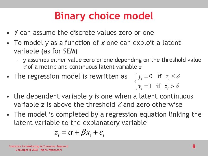 Binary choice model • Y can assume the discrete values zero or one • To model y as a function of x one can exploit a latent variable (as for SEM) – y assumes either value zero or one depending on the threshold value d of a metric and continuous latent variable z • The regression model is rewritten as • the dependent variable y is one when a latent continuous variable z is above threshold d and zero otherwise • The model is completed by a regression equation linking the latent variable to the explanatory variable Statistics for Marketing & Consumer Research Copyright © 2008 - Mario Mazzocchi 8
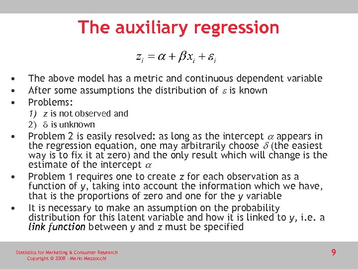 The auxiliary regression • • • The above model has a metric and continuous dependent variable After some assumptions the distribution of e is known Problems: 1) z is not observed and 2) d is unknown • • • Problem 2 is easily resolved: as long as the intercept a appears in the regression equation, one may arbitrarily choose d (the easiest way is to fix it at zero) and the only result which will change is the estimate of the intercept a Problem 1 requires one to create z for each observation as a function of y, taking into account the information which we have, that is the proportions of zero and one for the y variable It is necessary to make an assumption on the probability distribution for this latent variable and how it is linked to y, i. e. a link function between y and z must be specified Statistics for Marketing & Consumer Research Copyright © 2008 - Mario Mazzocchi 9
 The link functions • The link function specifies the relationship between z and y through the expected value of the appropriate distribution function for the generic observation yi • For example, with binary data, one can assume that the probabilities of each observation yi follow a binomial distribution • there a number of transformations of y which create a z variable compatible with the binomial distribution Statistics for Marketing & Consumer Research Copyright © 2008 - Mario Mazzocchi 10
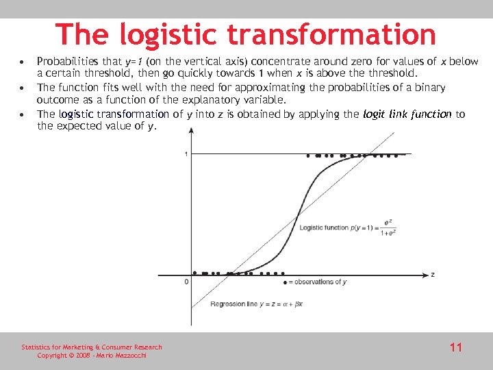 The logistic transformation • • • Probabilities that y=1 (on the vertical axis) concentrate around zero for values of x below a certain threshold, then go quickly towards 1 when x is above threshold. The function fits well with the need for approximating the probabilities of a binary outcome as a function of the explanatory variable. The logistic transformation of y into z is obtained by applying the logit link function to the expected value of y. Statistics for Marketing & Consumer Research Copyright © 2008 - Mario Mazzocchi 11
 Logistic regression • The logit transformation is the link function for logistic regression • The logit transformation is the log of the odds that y=1 relative to y=0 • The logit link allows to transform the binary variable y into a continuous variable z • The final equation is a regression model with a continuous variable on the left-hand side • The only difference from the standard regression model is that the distribution of the error is not normal but logistic. • Estimation of a and b can be obtained by maximum likelihood which works with any known probability distribution of the errors and returns the maximum likelihood estimates (the most probable values for the parameters) Statistics for Marketing & Consumer Research Copyright © 2008 - Mario Mazzocchi 12
 Types of discrete choice models • Logistic regression: at least one of the explanatory variables is metric and continuous • Logit model: all of the variables on the right-hand side are non-metric (binary or categorical) • This is a conventional distinction; often the two terms are used interchangeably • In a logit model with a categorical or binary x variable, the coefficient b is mathematically related to the odds ratio (with respect to the baseline category of x) of having a positive outcome – For example, if the dependent variable is one when the consumer buys a specific brand x measures whether the consumer has kids or not, one can compute with eb the odds ratio of buying the brand for consumers with kids as compared to consumers without kids. Statistics for Marketing & Consumer Research Copyright © 2008 - Mario Mazzocchi 13
 Probit model • The Probit model is also applied to binary dependent variables but with different assumptions on the link function and the error distribution • The link function (called probit) is the inverse of the standard normal cumulative distribution function • This link function guarantees that the distribution of the model which is finally estimated is still normal • The choice between the probit and the logit distribution depends on the type of dependent variable • if the dependent variable can be reasonably assumed to be a proxy for a true underlying variable which is normally distributed then the probit model should be chosen • if the dependent variable is considered to be a truly qualitative and binomial character then logit modelling should be preferred • generally the two models lead to very similar results, unless cases are concentrated to the tails of the distributions in which case the logit link function should be chosen Statistics for Marketing & Consumer Research Copyright © 2008 - Mario Mazzocchi 14
 Generalizations • ordered logit (ordered probit) models • the dependent variable is not binary but categorical and the categories are ordered • multinomial logit (multinomial probit) • The dependent variable is categorical but categories cannot be ordered • multivariate logit (multivariate probit) • Several discrete choice models are estimated simultaneously (there are multiple dependent variable) Statistics for Marketing & Consumer Research Copyright © 2008 - Mario Mazzocchi 15
 Discrete choice models in SPSS • Trust data-set • Binary logistic regression • Example application (as for discriminant analysis) • Dependent variable: buying chicken at the butcher’s shop • Explanatory variables: • • weekly expenditure on chicken age safety of butcher’s chicken trust in supermarkets Statistics for Marketing & Consumer Research Copyright © 2008 - Mario Mazzocchi 16
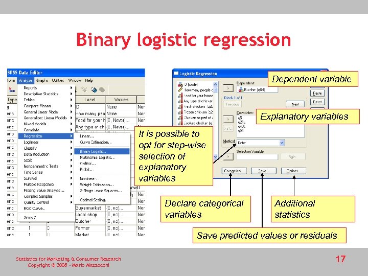 Binary logistic regression Dependent variable Explanatory variables It is possible to opt for step-wise selection of explanatory variables Declare categorical variables Additional statistics Save predicted values or residuals Statistics for Marketing & Consumer Research Copyright © 2008 - Mario Mazzocchi 17
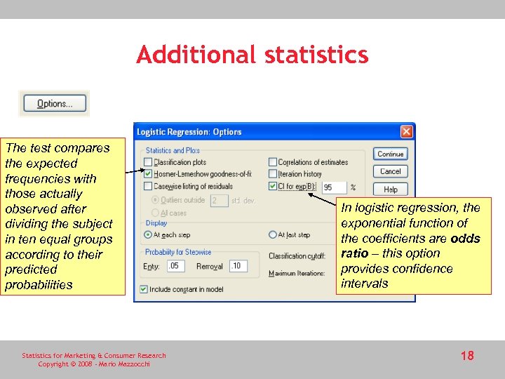 Additional statistics The test compares the expected frequencies with those actually observed after dividing the subject in ten equal groups according to their predicted probabilities Statistics for Marketing & Consumer Research Copyright © 2008 - Mario Mazzocchi In logistic regression, the exponential function of the coefficients are odds ratio – this option provides confidence intervals 18
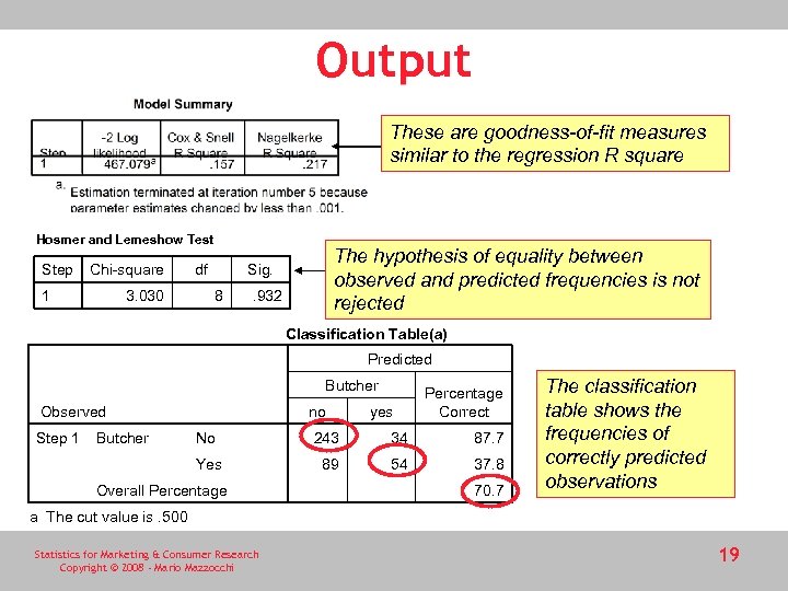 Output These are goodness-of-fit measures similar to the regression R square Hosmer and Lemeshow Test Step Chi-square 1 3. 030 df The hypothesis of equality between observed and predicted frequencies is not rejected Sig. 8 . 932 Classification Table(a) Predicted Butcher no Observed Step 1 Butcher yes Percentage Correct No 243 34 87. 7 Yes 89 54 37. 8 Overall Percentage 70. 7 The classification table shows the frequencies of correctly predicted observations a The cut value is. 500 Statistics for Marketing & Consumer Research Copyright © 2008 - Mario Mazzocchi 19
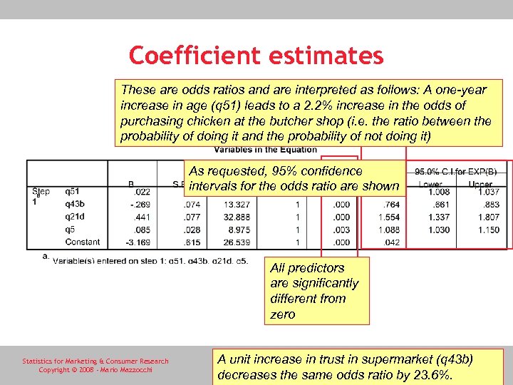 Coefficient estimates These are odds ratios and are interpreted as follows: A one-year increase in age (q 51) leads to a 2. 2% increase in the odds of purchasing chicken at the butcher shop (i. e. the ratio between the probability of doing it and the probability of not doing it) As requested, 95% confidence intervals for the odds ratio are shown All predictors are significantly different from zero Statistics for Marketing & Consumer Research Copyright © 2008 - Mario Mazzocchi A unit increase in trust in supermarket (q 43 b) 20 decreases the same odds ratio by 23. 6%.
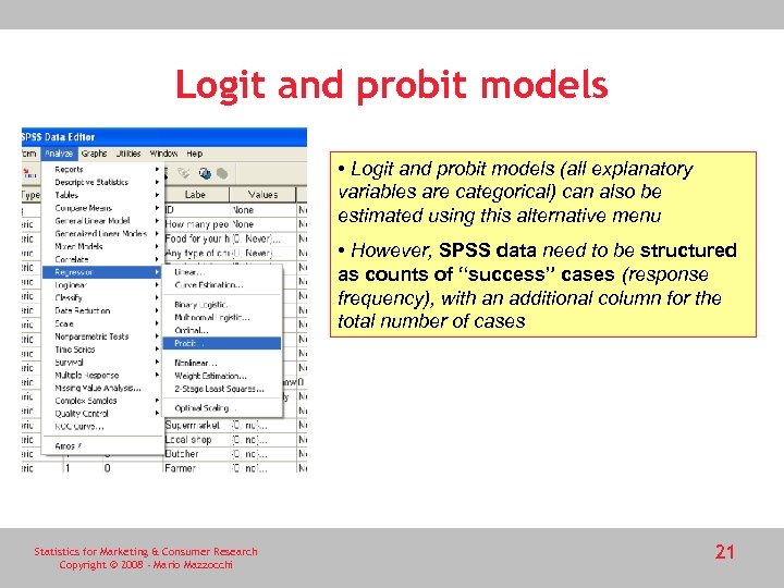 Logit and probit models • Logit and probit models (all explanatory variables are categorical) can also be estimated using this alternative menu • However, SPSS data need to be structured as counts of “success” cases (response frequency), with an additional column for the total number of cases Statistics for Marketing & Consumer Research Copyright © 2008 - Mario Mazzocchi 21
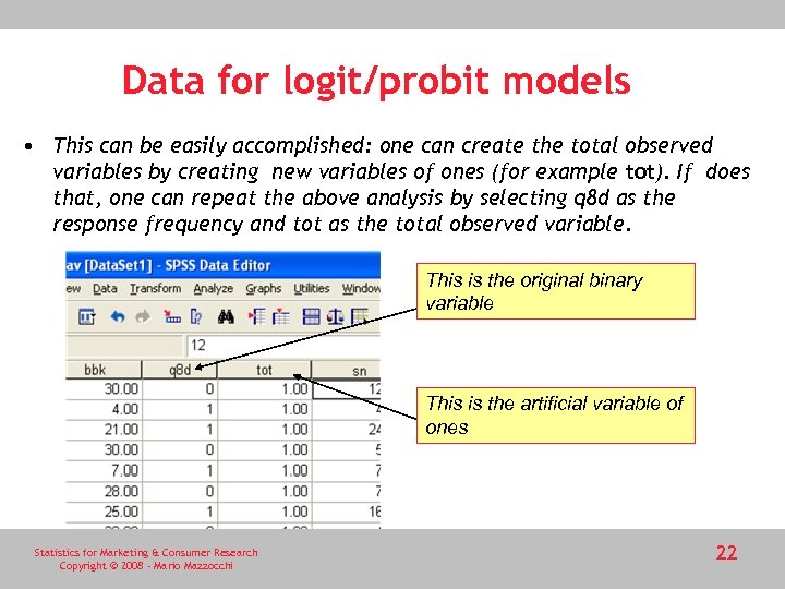 Data for logit/probit models • This can be easily accomplished: one can create the total observed variables by creating new variables of ones (for example tot). If does that, one can repeat the above analysis by selecting q 8 d as the response frequency and tot as the total observed variable. This is the original binary variable This is the artificial variable of ones Statistics for Marketing & Consumer Research Copyright © 2008 - Mario Mazzocchi 22
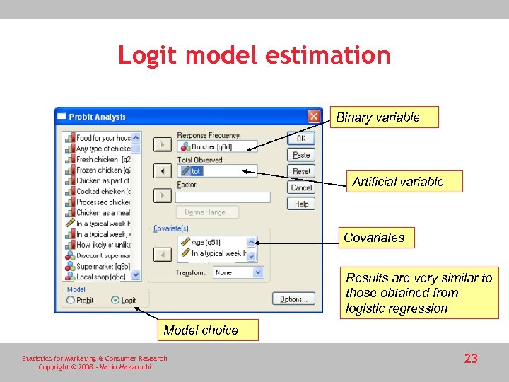 Logit model estimation Binary variable Artificial variable Covariates Results are very similar to those obtained from logistic regression Model choice Statistics for Marketing & Consumer Research Copyright © 2008 - Mario Mazzocchi 23
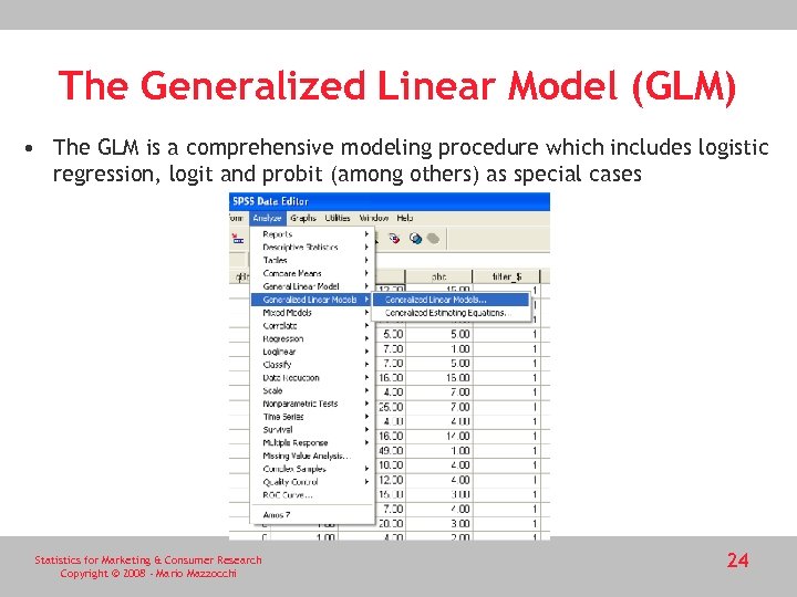 The Generalized Linear Model (GLM) • The GLM is a comprehensive modeling procedure which includes logistic regression, logit and probit (among others) as special cases Statistics for Marketing & Consumer Research Copyright © 2008 - Mario Mazzocchi 24
 GLM • It is comprehensive modeling approach for discrete choice modeling where one or more dependent categorical variables are modeled as the outcome of one or more explanatory variables which can be metric or non-metric. • Depending on the type of link function the GLM collapses into: • logistic regression • logit or probit models • multinomial or multivariate logistic regression logit or probit models Statistics for Marketing & Consumer Research Copyright © 2008 - Mario Mazzocchi 25
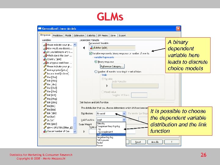 GLMs A binary dependent variable here leads to discrete choice models It is possible to choose the dependent variable distribution and the link function Statistics for Marketing & Consumer Research Copyright © 2008 - Mario Mazzocchi 26
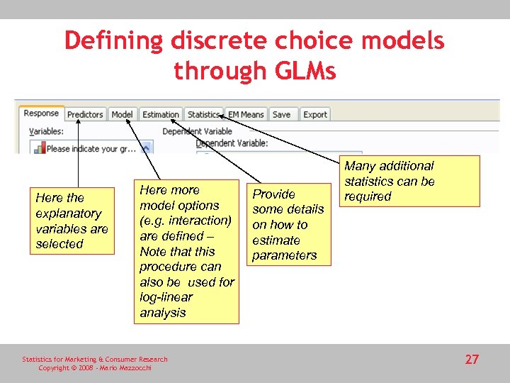 Defining discrete choice models through GLMs Here the explanatory variables are selected Here model options (e. g. interaction) are defined – Note that this procedure can also be used for log-linear analysis Statistics for Marketing & Consumer Research Copyright © 2008 - Mario Mazzocchi Provide some details on how to estimate parameters Many additional statistics can be required 27
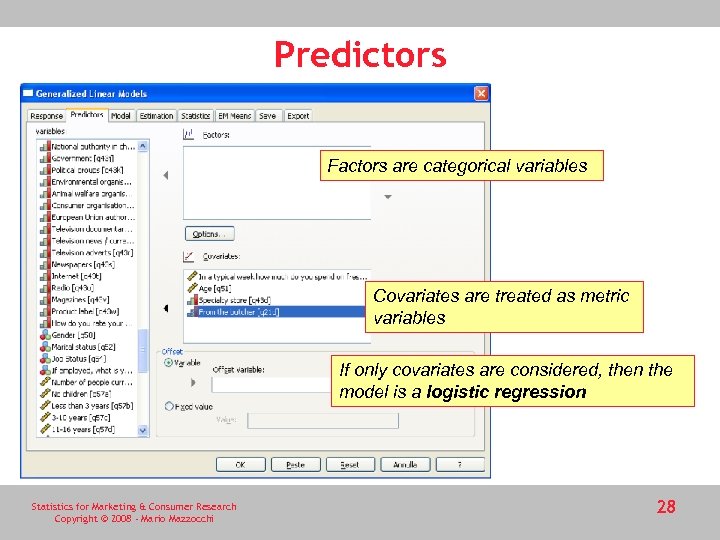 Predictors Factors are categorical variables Covariates are treated as metric variables If only covariates are considered, then the model is a logistic regression Statistics for Marketing & Consumer Research Copyright © 2008 - Mario Mazzocchi 28
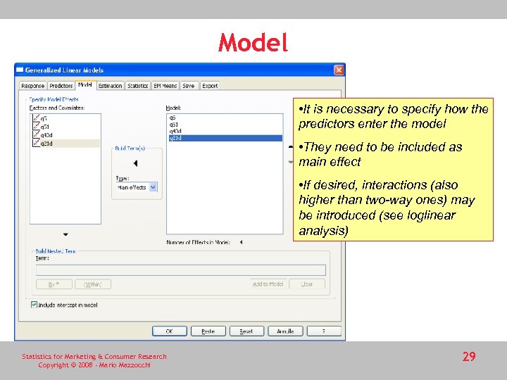 Model • It is necessary to specify how the predictors enter the model • They need to be included as main effect • If desired, interactions (also higher than two-way ones) may be introduced (see loglinear analysis) Statistics for Marketing & Consumer Research Copyright © 2008 - Mario Mazzocchi 29
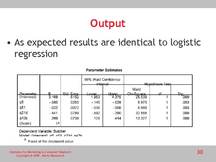 Output • As expected results are identical to logistic regression Statistics for Marketing & Consumer Research Copyright © 2008 - Mario Mazzocchi 30
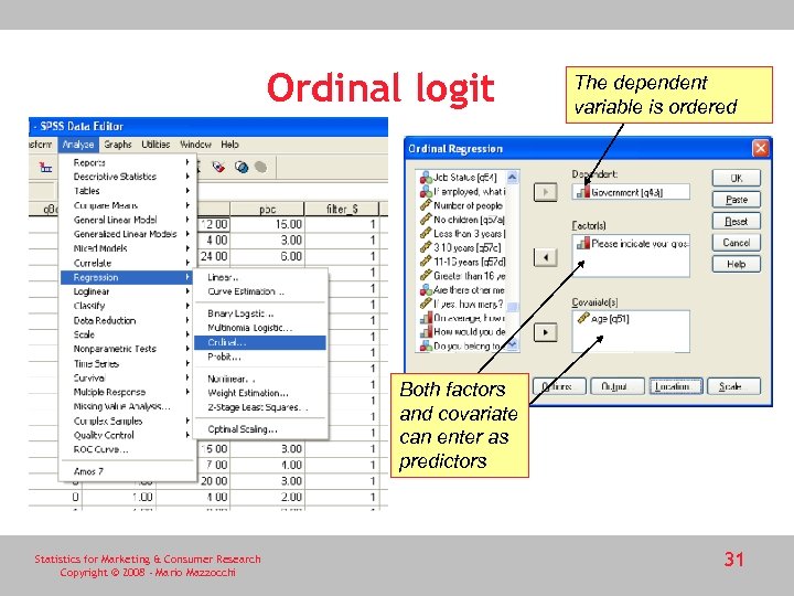 Ordinal logit The dependent variable is ordered Both factors and covariate can enter as predictors Statistics for Marketing & Consumer Research Copyright © 2008 - Mario Mazzocchi 31
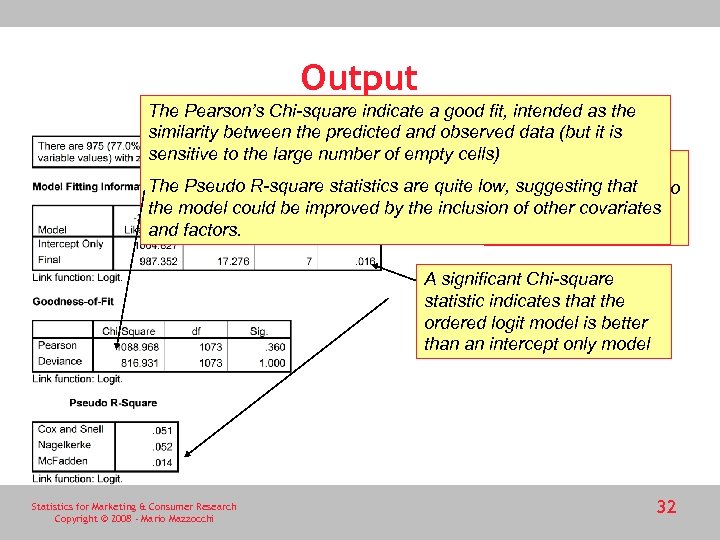 Output The Pearson’s Chi-square indicate a good fit, intended as the similarity between the predicted and observed data (but it is sensitive to the large number of empty cells) A large proportion of The Pseudo R-square statistics are quite low, suggesting that empty cells may lead to the model could be improved by the inclusion of other covariates invalid goodness-of-fit and factors. measures A significant Chi-square statistic indicates that the ordered logit model is better than an intercept only model Statistics for Marketing & Consumer Research Copyright © 2008 - Mario Mazzocchi 32
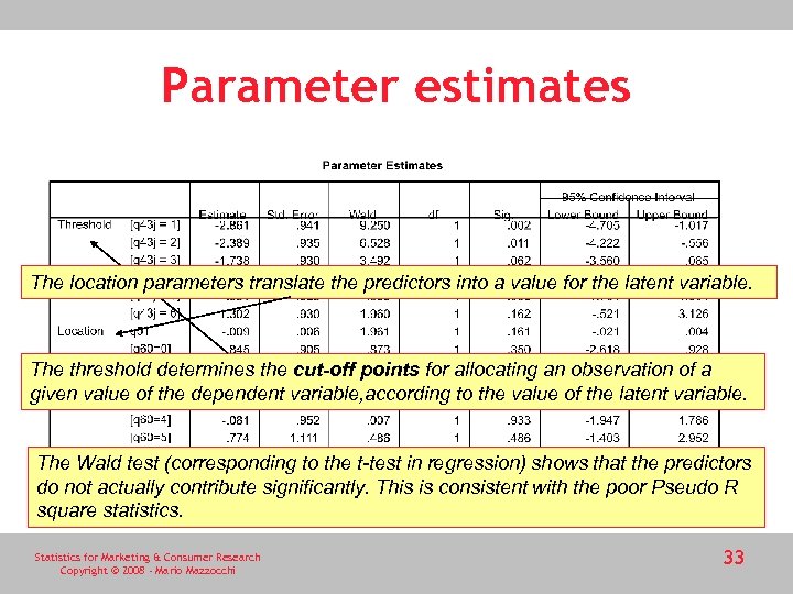 Parameter estimates The location parameters translate the predictors into a value for the latent variable. The threshold determines the cut-off points for allocating an observation of a given value of the dependent variable, according to the value of the latent variable. The Wald test (corresponding to the t-test in regression) shows that the predictors do not actually contribute significantly. This is consistent with the poor Pseudo R square statistics. Statistics for Marketing & Consumer Research Copyright © 2008 - Mario Mazzocchi 33
 Marginal effects • What could be interesting (at least for a model with a better fit) is the computation of the marginal effects • They represent the change in the probability of an observation of being classified in each specific category of the dependent variable according to the values of the predictors • Unfortunately SPSS does not provide marginal effects Statistics for Marketing & Consumer Research Copyright © 2008 - Mario Mazzocchi 34
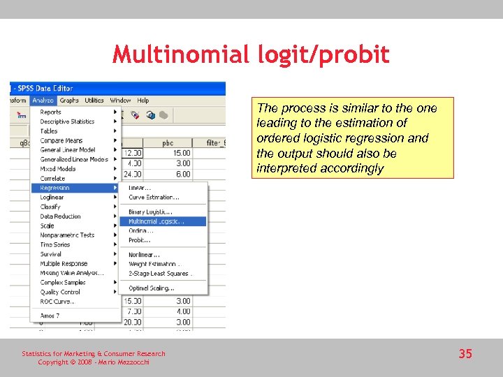 Multinomial logit/probit The process is similar to the one leading to the estimation of ordered logistic regression and the output should also be interpreted accordingly Statistics for Marketing & Consumer Research Copyright © 2008 - Mario Mazzocchi 35
 Statistical packages for discrete choice models • SPSS lacks some useful features like the estimation of marginal effects • In SAS discrete choice models can be estimated with several procedures in SAS/STAT – CATMOD is employed for estimating logistic regression when the data are structured as a frequency table – Binary and ordinal logistic regression can be obtained through the procedure LOGISTIC – The same models can be estimated with the PROBIT procedure which also enables estimation of probit models. – GENMOD allows one to specify a variety of link functions for generalized linear models • LIMDEP was specifically created for the estimation of limited dependent variable models, which include discrete choice models – It is extremely flexible and contains all the required features and the most up-todate diagnostics • STATA estimates discrete choice models with marginal effects • Econometric views allow estimation of discrete choice models but the availability of diagnostics is rather limited when compared to Lim. Dep and no marginal effects are displayed. Statistics for Marketing & Consumer Research Copyright © 2008 - Mario Mazzocchi 36
 Conjoint analysis • Very popular research technique in marketing closely associated with stated preference analysis • Mainly exploited for the development of new products and the modification of product characteristics • Conjoint analysis is not a model or an estimation technique but rather a methodology for constructing the data collection instrument when the final objective is choice modeling Statistics for Marketing & Consumer Research Copyright © 2008 - Mario Mazzocchi 37
 Marketing applications of conjoint analysis • The most common application in consumer research is the analysis of consumer evaluations of different combinations of product attributes • Example • A car manufacturer needs to take some decision about some options to be provided for car configuration • range of colours • model of car stereo • presence of air conditioning, etc. • Rather than asking consumers about their evaluation of these attributes on a one-by-one basis, conjoint analysis starts by creating potential combinations of the product attributes • E. g. • Combination 1: red car, with an mp 3 stereo player and no air-conditioning, • Combination 2: red car, but with a standard CD player and air-conditioning, etc. • Respondents choose among these alternative potential products defined by the combination of attributes • From the final choice, conjoint analysis elicits the relevance of each attribute Statistics for Marketing & Consumer Research Copyright © 2008 - Mario Mazzocchi 38
 Conjoint analysis • When several attributes are considered simultaneously the number of potential combinations is quite high • Conjoint analysis creates many different choice sets each one containing a limited number of options • Conjoint analysis is based on the statistical control of • the way choices are allocated in the sample • the distribution of attributes • Hence, the collected data enable inference on preferences and evaluations for the individual attributes Statistics for Marketing & Consumer Research Copyright © 2008 - Mario Mazzocchi 39
 Theoretical basis for conjoint analysis • The underlying theory for conjoint analysis is based on the economic concept of utility • each individual has a specific set of preferences for bundles of products (and attributes) • individuals take decisions in a way to maximize the level of satisfaction from consumption (the utility level) • By observing many individuals it is possible to go back from stated choices to preferences • Conjoint analysis is inspired by scientific experimental designs and the terminology reflects this association • Attributes are called factors (e. g. car colour) • The different values factors can assume are the levels (red, blue, yellow, etc. ) Statistics for Marketing & Consumer Research Copyright © 2008 - Mario Mazzocchi 40
 Factors and choice sets • An additional factor could be the price of the car • By including price levels in the choice set it becomes possible to evaluate how much consumers would be willing to pay for the car they prefer • Among the potential set of choices there are some nonsense choices e. g. including all car options but setting a very low price • Nonsense choices can be excluded by the researcher who has control on the overall choice set • Questionnaire • Respondents must choose from the preferred combination of attributes or • Respondents must rank all possible choices according to their preferences • Conjoint analysis is a decompositional method (recall multidimensional scaling techniques), as it starts from an overall evaluation to infer preferences for the individual product attributes Statistics for Marketing & Consumer Research Copyright © 2008 - Mario Mazzocchi 41
 Theories attributes and choice • The experimental design and the modeling of preferences depend on theories which link the evaluation of single attributes to the final choice • part-worth model: assumes that total utility of a choice is equal to the sum of utilities of the attributes of that specific choice • vector linear model: applicable when all attributes are measured on a metric (continuous) scale, assumes a linear relationship between the utility of individual attributes and total utility • ideal point model: assumes that the consumer has an ideal level for all factors and the total utility depends upon the distance between the actual levels and the ideal levels Statistics for Marketing & Consumer Research Copyright © 2008 - Mario Mazzocchi 42
 Experimental design • The key problem of conjoint analysis is the large number of alternative combinations of attributes which arise when there are many factors and levels • E. g. a product with six attributes, each with three levels potentially allows for 729 different combinations • It would be unrealistic to assume that respondents are able to choose among so many alternatives • This problem can be solved by an appropriate experimental design • Objective: understand the relationship between the factors and the potential choice with a number of observations as small as possible • The experimental design sets the criteria to obtain the preference information from an aggregation of respondents (full factorial designs: all potential products are compared (729 in the example)) • fractional factorial designs: exploits the experimental design to reduce the number of choices, still guaranteeing that the sample will produce meaningful aggregate results Statistics for Marketing & Consumer Research Copyright © 2008 - Mario Mazzocchi 43
 Types of conjoint analyses • Traditional conjoint analysis – each respondent is faced with the whole set of attributes – it requires either a full factorial design or a fractional factorial design – all attributes appear in the choice set of each respondent (although not for all levels) – becomes inapplicable as the number of factors or levels increases • Adaptive conjoint analysis – these design issues are dealt with – each respondent only deals with a sub-set of potential choices – these sub-set can be defined in different ways. For example: respondents could be asked to rank the factors first, then the ranking is exploited to adapt data collection – Computer software learns from the earlier responses and builds the data-sets accordingly Statistics for Marketing & Consumer Research Copyright © 2008 - Mario Mazzocchi 44
 Choice-based conjoint (1) • The decomposition of the observed choices into weights and preferences for single attributes is generally obtained for an aggregate of consumers or for homogeneous groups of consumers • Several techniques can be employed for this purpose • The evolution of discrete choice models has given relevance to a specific type of adaptive conjoint analysis, choice-based conjoint • Choice-based conjoint gives the respondent the possibility of evaluating all attributes, not in a single (often too complex) choice, but rather within a sequence of smaller choice sets where the possibility of choosing none of the alternatives is also given Statistics for Marketing & Consumer Research Copyright © 2008 - Mario Mazzocchi 45
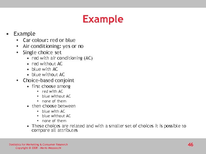 Example • Car colour: red or blue • Air conditioning: yes or no • Single choice set • • red with air conditioning (AC) red without AC blue without AC • Choice-based conjoint • first choose among • red with AC • blue without AC • none of them • then choose between • blue with AC • blue without AC • none of them • These choices are related and with a smaller set of choices it is possible to compare all attributes Statistics for Marketing & Consumer Research Copyright © 2008 - Mario Mazzocchi 46
 Choice-based conjoint (2) • The advantages of choice-based conjoint are apparent with complex cases • Respondents do not need to compare too many stimuli at once, • They face a more realistic choice among a limited set of alternatives • With many factors and levels, each respondent can be asked to face a limited number of choice sets • The sufficient condition is that an homogeneous group of respondents (i. e. respondents that are similar in terms of characteristics that can influence the choice) is confronted with the whole range of alternatives, then the estimation technique will do the rest Statistics for Marketing & Consumer Research Copyright © 2008 - Mario Mazzocchi 47
 Estimation and models • The experimental design is at the core of a successful choice-based conjoint • There is an evolving research effort to guarantee the quality of the analysis • Once the data has been collected the natural estimation technique is the multinomial logit • choices represent the categorical dependent variable and the attribute levels are the explanatory variables • There are computer packages specifically developed for conjoint analysis • SPSS Conjoint module • deals with the experimental design • provides estimates based on an orthogonal decomposition of the design matrix • In SAS/STAT, the TRANSREG procedure is a useful support to define the experimental design Statistics for Marketing & Consumer Research Copyright © 2008 - Mario Mazzocchi 48


