

6e3fe4833beafe433f8f2b96f33c33d4.ppt
- Количество слайдов: 80
 Discrete Choice Modeling William Greene Stern School of Business IFS at UCL February 11 -13, 2004
 Discrete Choice Modeling o Econometric Methodology n n o Model Building n n o Binary Choice Models Multinomial Choice Specification Estimation Analysis Applications NLOGIT Software
 Our Agenda 1. 2. 3. 4. 5. 6. 7. 8. 9. 10. 11. 12. Methodology Discrete Choice Models Binary Choice Models Panel Data Models for Binary Choice Introduction to NLOGIT Discrete Choice Settings The Multinomial Logit Model Heteroscedasticity in Utility Functions Nested Logit Modeling Latent Class Models Mixed Logit Models and Simulation Based Estimation Revealed and Stated Preference Data Sets
 Part 1 Methodology
 Measurement as Observation Population Theory Measurement Characteristics Behavior Patterns
 Individual Behavioral Modeling o Assumptions about behavior n n o Common elements across individuals Unique elements Prediction n n Population aggregates Individual behavior
 Modeling Choice o o Activity as choices Preferences Behavioral axioms Choice as utility maximization
 Inference Population Econometrics Measurement Characteristics Behavior Patterns Choices
 Bayesian") Econometric Frameworks o o Nonparametric Parametric n n Classical (Sampling Theory) Bayesian
Econometric Frameworks o o Nonparametric Parametric n n Classical (Sampling Theory) Bayesian
 Likelihood Based Inference Methods Behavioral Theory Statistical Theory Observed Measurement Likelihood Function The likelihood function embodies theoretical description of the population. Characteristics of the population are inferred from the characteristics of the likelihood function. (Bayesian and Classical)
 Modeling Discrete Choice o o Theoretical foundations Econometric methodology n n n o o Models Statistical bases Econometric methods Estimation with econometric software Applications
 Part 2 Basics of Discrete Choice Modeling
 Modeling Consumer Choice: Continuous Measurement Example: Travel expenditure based on price and income Expenditure • What do we measure? Low price High price • What is revealed by the data? • What is the underlying model? • What are the empirical tools? Income
 Discrete Choice o Observed outcomes n n o Inherently discrete: number of occurrences (e. g. , family size; considered separately) Implicitly continuous: the observed data are discrete by construction (e. g. , revealed preferences; our main subject) Implications n n For model building For analysis and prediction of behavior
 Two Fundamental Building Blocks o Underlying Behavioral Theory: Random utility model The link between underlying behavior and observed data o Empirical Tool: Stochastic, parametric model for binary choice A platform for models of discrete choice
 Random Utility A Theoretical Proposition About Behavior o o o Consumer making a choice among several alternatives Example, brand choice (car, food) Choice setting for a consumer: Notation Consumer i, i = 1, …, N Choice setting t, t = 1, …, Ti (may be one) Choice set j, j = 1, …, Ji (may be fixed)
 Behavioral Assumptions Preferences are transitive and complete wrt choice situations o Utility is defined over alternatives: Uijt o Utility maximization assumption If Ui 1 t > Ui 2 t, consumer chooses alternative 1, not alternative 2. o Revealed preference (duality) If the consumer chooses alternative 1 and not alternative 2, then Ui 1 t > Ui 2 t. o
 Random Utility Functions Uitj = j + i ’xitj + i’zit + ijt j xitj = Choice specific constant i = Person specific taste weights zit i = Characteristics of the person ijt = Unobserved random component of utility = Attributes of choice presented to person = Weights on person specific characteristics Mean: E[ ijt] = 0, Var[ ijt] = 1
 Part 3 Modeling Binary Choice
 Example,") A Model for Binary Choice o o Yes or No decision (Buy/Not buy) Example, choose to fly or not to fly to a destination when there alternatives. Model: Net utility of flying Ufly = + 1 Cost + 2 Time + Income + Choose to fly if net utility is positive Data: X = [1, cost, terminal time] Z = [income] y = 1 if choose fly, Ufly > 0, 0 if not.
A Model for Binary Choice o o Yes or No decision (Buy/Not buy) Example, choose to fly or not to fly to a destination when there alternatives. Model: Net utility of flying Ufly = + 1 Cost + 2 Time + Income + Choose to fly if net utility is positive Data: X = [1, cost, terminal time] Z = [income] y = 1 if choose fly, Ufly > 0, 0 if not.
 What Can Be Learned from the Data? (A Sample of Consumers, i = 1, …, N) • Are the attributes “relevant? ” • Predicting behavior - Individual - Aggregate • Analyze changes in behavior when attributes change
 Application o o o 210 Commuters Between Sydney and Melbourne Available modes = Air, Train, Bus, Car Observed: n n n o Choice Attributes: Cost, terminal time, other Characteristics: Household income First application: Fly or other
 Binary Choice Data Choose Air 1. 00000 1. 00000 Gen. Cost 86. 000 67. 000 77. 000 69. 000 77. 000 71. 000 58. 000 71. 000 100. 00 158. 00 136. 00 103. 00 77. 000 197. 00 129. 00 123. 00 Term Time 25. 000 69. 000 64. 000 30. 000 45. 000 30. 000 69. 000 45. 000 64. 000 Income 70. 000 60. 000 20. 000 15. 000 30. 000 26. 000 35. 000 12. 000 70. 000 50. 000 40. 000 70. 000 10. 000 26. 000 50. 000 70. 000
 An Econometric Model o Choose to fly iff UFLY > 0 Ufly = + 1 Cost + 2 Time + Income + n Ufly > 0 > -( + 1 Cost + 2 Time + Income) n o Probability model: For any person observed by the analyst, Prob(fly) = Prob[ > -( + 1 Cost + 2 Time + Income)] o Note the relationship between the unobserved and the outcome
 + 1 Cost + 2 TTime + Income
 Econometrics o How to estimate , 1, 2, ? n It’s not regression The technique of maximum likelihood n Prob[y=1] = n Prob[ > -( + 1 Cost + 2 Time + Income)] Prob[y=0] = 1 - Prob[y=1] o Requires a model for the probability
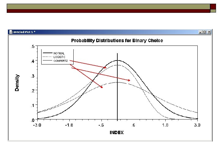
 o The distribution n o Normal: PROBIT, natural for") Completing the Model: F( ) o The distribution n o Normal: PROBIT, natural for behavior Logistic: LOGIT, allows “thicker tails” Gompertz: EXTREME VALUE, asymmetric, underlies the basic logit model for multiple choice Does it matter? n n Yes, large difference in estimates Not much, quantities of interest are more stable.
Completing the Model: F( ) o The distribution n o Normal: PROBIT, natural for behavior Logistic: LOGIT, allows “thicker tails” Gompertz: EXTREME VALUE, asymmetric, underlies the basic logit model for multiple choice Does it matter? n n Yes, large difference in estimates Not much, quantities of interest are more stable.
 Estimated Binary Choice Models LOGIT Variable Estimate Constant 1. 78458 GC 0. 0214688 TTME HINC -0. 098467 0. 0223234 PROBIT t-ratio EXTREME VALUE Estimate t-ratio 1. 40591 0. 438772 0. 702406 1. 45189 1. 34775 3. 15342 0. 012563 3. 41314 0. 0177719 3. 14153 -0. 0477826 -6. 65089 -0. 0868632 -5. 91658 -5. 9612 2. 16781 0. 0144224 2. 51264 0. 0176815 2. 02876 Log-L -80. 9658 -84. 0917 -76. 5422 Log-L(0) -123. 757
 Effect on predicted probability of an increase in income + 1 Cost + 2 Time + (Income+1) ( is positive)
![Marginal Effects in Probability Models Prob[Outcome] = some F( + 1 Cost…) o “Partial](https://present5.com/presentation/6e3fe4833beafe433f8f2b96f33c33d4/image-31.jpg "Marginal Effects in Probability Models Prob[Outcome] = some F( + 1 Cost…) o “Partial") Marginal Effects in Probability Models Prob[Outcome] = some F( + 1 Cost…) o “Partial effect” = F( + 1 Cost…) / ”x” (derivative) o n n Partial effects are derivatives Result varies with model o o n Logit: F( + 1 Cost…) / x = Prob * (1 -Prob) * Probit: F( + 1 Cost…) / x = Normal density Scaling usually erases model differences
Marginal Effects in Probability Models Prob[Outcome] = some F( + 1 Cost…) o “Partial effect” = F( + 1 Cost…) / ”x” (derivative) o n n Partial effects are derivatives Result varies with model o o n Logit: F( + 1 Cost…) / x = Prob * (1 -Prob) * Probit: F( + 1 Cost…) / x = Normal density Scaling usually erases model differences
 The Delta Method
 Marginal Effects for Binary Choice o Logit o Probit
 Estimated Marginal Effects Logit Estimate GC t-ratio Probit Estimate t-ratio Extreme Value Estimate t-ratio . 003721 3. 267 . 003954 3. 466 . 003393 3. 354 TTME -. 017065 -5. 042 -. 015039 -5. 754 -. 016582 -4. 871 HINC . 003869 2. 193 . 004539 2. 532 . 033753 2. 064
![Marginal Effect for a Dummy Variable Prob[yi = 1|xi, di] = F( ’xi+ di)](https://present5.com/presentation/6e3fe4833beafe433f8f2b96f33c33d4/image-35.jpg "Marginal Effect for a Dummy Variable Prob[yi = 1|xi, di] = F( ’xi+ di)") Marginal Effect for a Dummy Variable Prob[yi = 1|xi, di] = F( ’xi+ di) =conditional mean o Marginal effect of d Prob[yi = 1|xi, di=1]=Prob[yi= 1|xi, di=0] o Logit: o
Marginal Effect for a Dummy Variable Prob[yi = 1|xi, di] = F( ’xi+ di) =conditional mean o Marginal effect of d Prob[yi = 1|xi, di=1]=Prob[yi= 1|xi, di=0] o Logit: o
 Effect – Dummy Variable o High. Incm = 1(Income > 50) +----------------------+ |") (Marginal) Effect – Dummy Variable o High. Incm = 1(Income > 50) +----------------------+ | Partial derivatives of probabilities with | | respect to the vector of characteristics. | | They are computed at the means of the Xs. | | Observations used are All Obs. | +----------------------+ +--------------+--------+---------+-----+ |Variable | Coefficient | Standard Error |b/St. Er. |P[|Z|>z] | Mean of X| +--------------+--------+---------+-----+ Characteristics in numerator of Prob[Y = 1] Constant. 4750039483. 23727762 2. 002. 0453 GC. 3598131572 E-02. 11354298 E-02 3. 169. 0015 102. 64762 TTME -. 1759234212 E-01. 34866343 E-02 -5. 046. 0000 61. 009524 Marginal effect for dummy variable is P|1 - P|0. HIGHINCM. 8565367181 E-01. 99346656 E-01. 862. 3886 (Autodetected) . 18571429
(Marginal) Effect – Dummy Variable o High. Incm = 1(Income > 50) +----------------------+ | Partial derivatives of probabilities with | | respect to the vector of characteristics. | | They are computed at the means of the Xs. | | Observations used are All Obs. | +----------------------+ +--------------+--------+---------+-----+ |Variable | Coefficient | Standard Error |b/St. Er. |P[|Z|>z] | Mean of X| +--------------+--------+---------+-----+ Characteristics in numerator of Prob[Y = 1] Constant. 4750039483. 23727762 2. 002. 0453 GC. 3598131572 E-02. 11354298 E-02 3. 169. 0015 102. 64762 TTME -. 1759234212 E-01. 34866343 E-02 -5. 046. 0000 61. 009524 Marginal effect for dummy variable is P|1 - P|0. HIGHINCM. 8565367181 E-01. 99346656 E-01. 862. 3886 (Autodetected) . 18571429
 Computing Effects o Compute at the data means? n n o Simple Inference is well defined Average individual effects n n More appropriate? Asymptotic standard errors. (Not done correctly in the literature – terms are correlated!)
 Elasticities o Elasticity = o How to compute standard errors? n n Delta method Bootstrap o o Bootstrap the individual elasticities? (Will neglect variation in parameter estimates. ) Bootstrap model estimation?
 Estimated Income Elasticity for Air Choice Model +---------------------+ | Results of bootstrap estimation of model. | | Model has been reestimated 25 times. | | Statistics shown below are centered | | around the original estimate based on | | the original full sample of observations. | | Result is ETA =. 71183 | | bootstrap samples have 840 observations. | | Estimate Rt. Mn. Sq. Dev Skewness Kurtosis | |. 712. 266 -. 779 2. 258 | | Minimum =. 125 Maximum = 1. 135 | +---------------------+ Mean Income = 34. 55, Mean P =. 2716, Estimated ME =. 004539, Estimated Elasticity=0. 5774.
 Odds Ratio – Logit Model Only o Effect Measure? “Effect of a unit change in the odds ratio. ”
 Inference for Odds Ratios o o Logit coefficient = , estimate = b Coefficient = exp( ), estimate = exp(b) Standard error = exp(b) times se(b) t ratio is the same
 How Well Does the Model Fit? o o There is no R squared “Fit measures” computed from log L n n o “pseudo R squared = 1 – log. L 0/log. L Others… - these do not measure fit. Direct assessment of the effectiveness of the model at predicting the outcome
 Fit Measures for Binary Choice o Likelihood Ratio Index n n o Bounded by 0 and 1 Rises when the model is expanded Cramer (and others)
 Fit Measures for the Logit Model +--------------------+ | Fit Measures for Binomial Choice Model | | Probit model for variable MODE | +--------------------+ | Proportions P 0=. 723810 P 1=. 276190 | | N = 210 N 0= 152 N 1= 58 | | Log. L = -84. 09172 Log. L 0 = -123. 7570 | | Estrella = 1 -(L/L 0)^(-2 L 0/n) =. 36583 | +--------------------+ | Efron | Mc. Fadden | Ben. /Lerman | |. 45620 |. 32051 |. 75897 | | Cramer | Veall/Zim. | Rsqrd_ML | |. 40834 |. 50682 |. 31461 | +--------------------+ | Information Akaike I. C. Schwarz I. C. | | Criteria. 83897 189. 57187 | +--------------------+
 Predicting the Outcome Predicted probabilities P = F(a + b 1 Cost + b 2 Time + c. Income) o Predicting outcomes o n n o Predict y=1 if P is large Use 0. 5 for “large” (more likely than not) Count successes and failures
![Individual Predictions from a Logit Model Observation Observed Y Predicted Y Residual x(i)b Pr[Y=1]](https://present5.com/presentation/6e3fe4833beafe433f8f2b96f33c33d4/image-46.jpg "Individual Predictions from a Logit Model Observation Observed Y Predicted Y Residual x(i)b Pr[Y=1]") Individual Predictions from a Logit Model Observation Observed Y Predicted Y Residual x(i)b Pr[Y=1] 81 . 00000 -3. 3944 . 0325 85 . 00000 -2. 1901 . 1006 89 1. 00000 1. 0000 -2. 6766 . 0644 93 1. 0000 . 8113 . 6924 97 1. 0000 2. 6845 . 9361 101 1. 0000 2. 4457 . 9202 105 1. 00000 1. 0000 -3. 2204 . 0384 109 1. 0000 . 0311 . 5078 113 . 00000 -2. 1704 . 1024 117 . 00000 -3. 3729 . 0332 445 . 00000 1. 0000 -1. 0000 . 0295 . 5074 Note two types of errors and two types of successes.
Individual Predictions from a Logit Model Observation Observed Y Predicted Y Residual x(i)b Pr[Y=1] 81 . 00000 -3. 3944 . 0325 85 . 00000 -2. 1901 . 1006 89 1. 00000 1. 0000 -2. 6766 . 0644 93 1. 0000 . 8113 . 6924 97 1. 0000 2. 6845 . 9361 101 1. 0000 2. 4457 . 9202 105 1. 00000 1. 0000 -3. 2204 . 0384 109 1. 0000 . 0311 . 5078 113 . 00000 -2. 1704 . 1024 117 . 00000 -3. 3729 . 0332 445 . 00000 1. 0000 -1. 0000 . 0295 . 5074 Note two types of errors and two types of successes.
 Predictions in Binary Choice Predict y = 1 if P > P* Success depends on the assumed P*
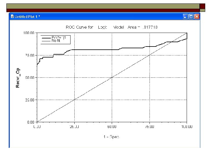
 ROC Curve o o o Plot %Y=1 correctly predicted vs. %y=1 incorrectly predicted 450 is no fit. Curvature implies fit. Area under the curve compares models
 Aggregate Predictions Frequencies of actual & predicted outcomes Predicted outcome has maximum probability. Threshold value for predicting Y=1 =. 5000 Predicted -----Actual ---------- + ----- 1 | Total ----- + ----- 0 0 151 1 | 152 1 20 38 | 58 ----- + ----- | 210 -----Total 171 39
 Analyzing Predictions Frequencies of actual & predicted outcomes Predicted outcome has maximum probability. Threshold value for predicting Y=1 is P*. 5000. (This table can be computed with any P*. ) Predicted -----Actual -------------0 1 + ----- | Total -----------+------- 0 N(a 0, p 0) N(a 0, p 1) | N(a 0) 1 N(a 1, p 0) N(a 1, p 1) | N(a 1) --------------+ ----- Total N(p 0) N N(p 1) |
 Analyzing Predictions - Success o Sensitivity = % actual 1 s correctly predicted = 100 N(a 1, p 1)/N(a 1) % [100(38/58)=65. 5%] o Specificity = % actual 0 s correctly predicted = 100 N(a 0, p 0)/N(a 0) % [100(151/152)=99. 3%] o Positive predictive value = % predicted 1 s that were actual 1 s = 100 N(a 1, p 1)/N(p 1) % [100(38/39)=97. 4%] o Negative predictive value = % predicted 0 s that were actual 0 s = 100 N(a 0, p 0)/N(p 0) % [100(151/171)=88. 3%] o Correct prediction = %actual 1 s and 0 s correctly predicted = 100[N(a 1, p 1)+N(a 0, p 0)]/N [100(151+38)/210=90. 0%]
 Analyzing Predictions - Failures o False positive for true negative = %actual 0 s predicted as 1 s = 100 N(a 0, p 1)/N(a 0) % [100(1/152)=0. 668%] o False negative for true positive = %actual 1 s predicted as 0 s = 100 N(a 1, p 0)/N(a 1) % [100(20/258)=34. 5%] o False positive for predicted positive = % predicted 1 s that were actual 0 s = 100 N(a 0, p 1)/N(p 1) % [100(1/39)=2/56%] o False negative for predicted negative = % predicted 0 s that were actual 1 s = 100 N(a 1, p 0)/N(p 0) % [100(20/171)=11. 7%] o False predictions = %actual 1 s and 0 s incorrectly predicted = 100[N(a 0, p 1)+N(a 1, p 0)]/N [100(1+20)/210=10. 0%]
 Aggregate Prediction is a Useful Way to Assess the Importance of a Variable Frequencies of actual & predicted outcomes. Predicted outcome has maximum probability. Threshold value for predicting Y=1 =. 5000 Predicted ---------- + ------ Actual 0 1 | Total Actual ---------- + ----- 1 | Total ----- + ----- 0 0 145 7 | 152 0 151 1 | 152 1 48 10 | 58 1 20 38 | 58 ---------- + ----- | 210 -----Total 193 17 Model fit without TTME -----Total 171 39 Model fit with TTME
 Simulating the Model to Examine Changes in Market Shares Suppose TTME increased by 25% for everyone. Before increase After increase Predicted -----Actual ------ + ------ 1 | Total Actual ----- + ------0 ----- + ----- 1 | Total ----- + ----- 0 0 151 1 | 152 0 | 152 1 20 38 | 58 1 29 29 | 58 ---------- + ----- | 210 -----Total 171 39 -----Total 181 29 • The model predicts 10 fewer people would fly • NOTE: The same model used for both sets of predictions.
 Scaling Uitj = j + i ’xitj + i’zit + ijt = Unobserved random component of utility o o Mean: E[ ijt] = 0, Var[ ijt] = 1 Why assume variance = 1? What if there are subgroups with different variances? n n o Cost of ignoring the between group variation? Specifically modeling More general heterogeneity across people n n Cost of the homogeneity assumption Modeling issues
 Choice Between Two Alternatives o By way of example: Automobile type n n Attribute: xij = price, perhaps others Characteristic: zi = income No variation in taste parameters, i = What do revealed choices tell us? n o Choices (1) SUV or (2) Sedan, Ji = 2 One choice situation: Ti = 1
 o o Modeling the Binary Choice Ui, suv = suv + Psuv + suv. Income + i, suv Ui, sed = sed + Psed + sed. Income + i, sed Chooses SUV: Ui, suv > Ui, sed Ui, suv - Ui, sed > 0 ( SUV- SED) + (PSUV-PSED) + ( SUV- sed)Income + i, suv - i, sed > 0 i > -[ + (PSUV-PSED) + Income]
![Probability Model for Choice Between Two Alternatives i > -[ + (PSUV-PSED) + Income]](https://present5.com/presentation/6e3fe4833beafe433f8f2b96f33c33d4/image-59.jpg "Probability Model for Choice Between Two Alternatives i > -[ + (PSUV-PSED) + Income]") Probability Model for Choice Between Two Alternatives i > -[ + (PSUV-PSED) + Income]
Probability Model for Choice Between Two Alternatives i > -[ + (PSUV-PSED) + Income]
 Individual vs. Grouped Data o o o Proportions and Frequencies Likelihood is the same Yji may be 1 s and 0 s, proportions, or frequencies for the two outcomes.
 Weighting and Choice Based Sampling o o Weighted log likelihood for all data types Endogenous weights for individual data “Biased” sampling – “Choice Based”
 Choice Based Sample Population Weight Air 27. 62% 14% 0. 5068 Ground 72. 38% 86% 1. 1882
 Choice Based Sampling Correction Maximize Weighted Log Likelihood o Covariance Matrix Adjustment V = H-1 G H-1 (all three weighted) H = Hessian G = Outer products of gradients • “Robust” covariance matrix (? ) (Above without weights. What is it robust to? ) o
 Effect of Choice Based Sampling Unweighted +--------------+--------+---------+ |Variable | Coefficient | Standard Error |b/St. Er. |P[|Z|>z] | +--------------+--------+---------+ Constant 1. 784582594 1. 2693459 1. 406. 1598 GC. 2146879786 E-01. 68080941 E-02 3. 153. 0016 TTME -. 9846704221 E-01. 16518003 E-01 -5. 961. 0000 HINC. 2232338915 E-01. 10297671 E-01 2. 168. 0302 +-----------------------+ | Weighting variable CBWT | | Corrected for Choice Based Sampling | +-----------------------+ +--------------+--------+---------+ |Variable | Coefficient | Standard Error |b/St. Er. |P[|Z|>z] | +--------------+--------+---------+ Constant 1. 014022236 1. 1786164. 860. 3896 GC. 2177810754 E-01. 63743831 E-02 3. 417. 0006 TTME -. 7434280587 E-01. 17721665 E-01 -4. 195. 0000 HINC. 2471679844 E-01. 95483369 E-02 2. 589. 0096
 Hypothesis Testing – Neyman/Pearson o Comparisons of Likelihood Functions n n o Likelihood Ratio Tests Lagrange Multiplier Tests Distance Measures: Wald Statistics (All to be demonstrated in the lab)
 Heteroscedasticity in Binary Choice Models o o o Random utility: Yi = 1 iff ’xi + i > 0 Resemblance to regression: How to accommodate heterogeneity in the random unobserved effects across individuals? Heteroscedasticity – different scaling n n Parameterize: Var[ i] = exp( ’zi) Reformulate probabilities o Probit: o Partial effects are now very complicated
 “Deadbeat” = 1") Application: Credit Data o o o Counts of major derogatory reports) “Deadbeat” = 1 if MAJORDRG > 0 Mean depends on AGE, INCOME, OWNRENT, SELFEMPLOYED Variance depends on AVGEXP, DEPENDT (average monthly expenditure, number of dependents) Probit model with heteroscedasticity
Application: Credit Data o o o Counts of major derogatory reports) “Deadbeat” = 1 if MAJORDRG > 0 Mean depends on AGE, INCOME, OWNRENT, SELFEMPLOYED Variance depends on AVGEXP, DEPENDT (average monthly expenditure, number of dependents) Probit model with heteroscedasticity
 Probit with Heteroscedasticity +-----------------------+ | Binomial Probit Model | | Dependent variable DEADBEAT | | Number of observations 1319 | | Log likelihood function -639. 3388 | | Restricted log likelihood -653. 3217 | | Chi-squared 27. 96596 | | Degrees of freedom 6 | | Significance level. 9535906 E-04 | +-----------------------+ +--------------+--------+---------+-----+ |Variable | Coefficient | Standard Error |b/St. Er. |P[|Z|>z] | Mean of X| +--------------+--------+---------+-----+ Index function for probability Constant -1. 272312665. 13598690 -9. 356. 0000 AGE. 1126209389 E-01. 40404726 E-02 2. 787. 0053 33. 213103 INCOME. 5286782288 E-01. 20239074 E-01 2. 612. 0090 3. 3653760 OWNRENT -. 2049230056. 88518106 E-01 -2. 315. 0206. 44048522 SELFEMPL. 1143040149. 13825044. 827. 4084. 68991660 E-01 Variance function AVGEXP -. 4768665802 E-03. 12613317 E-03 -3. 781. 0002 185. 05707 DEPNDT. 6880605703 E-02. 42546206 E-01. 162. 8715. 99393480 +----------------------+ | Partial derivatives of E[y] = F[*] with | | respect to the vector of characteristics. | | They are computed at the means of the Xs. | | Observations used for means are All Obs. | +----------------------+ +--------------+--------+---------+-----+ |Variable | Coefficient | Standard Error |b/St. Er. |P[|Z|>z] | Mean of X| +--------------+--------+---------+-----+ Index function for probability Constant -. 3768739381. 54283831 E-01 -6. 943. 0000 AGE. 3335964337 E-02. 12357954 E-02 2. 699. 0069 33. 213103 INCOME. 1566006938 E-01. 65292318 E-02 2. 398. 0165 3. 3653760 OWNRENT -. 6070059841 E-01. 24667682 E-01 -2. 461. 0139. 44048522 SELFEMPL. 3385819023 E-01. 41052591 E-01. 825. 4095. 68991660 E-01 Variance function AVGEXP -. 1133874143 E-03. 31868469 E-04 -3. 558. 0004 185. 05707 DEPNDT. 1636042704 E-02. 10080807 E-01. 162. 8711. 99393480
 Part 4 Panel Data Models for Binary Choice
 Panel Data and Binary Choice Models Uit o = + ’xit + Person i specific effect Fixed effects using “dummy” variables Uit = i + ’xit + it o Random effects using omitted heterogeneity Uit = + ’xit + ( it + vi) o Same outcome mechanism: Yit = [Uit > 0]
 Fixed and Random Effects Models o Fixed Effects n n n o Random Effects n n n o Robust to both specifications Inconvenient to compute (many parameters) Incidental parameters problem Inconsistent if correlated with X Small number of parameters Easier to compute Computation – available estimators
 Fixed Effects o Dummy variable coefficients Uit = i + ’xit + it o Can be done by “brute force” for 10, 000 s of individuals o F(. ) = appropriate probability for the observed outcome o Compute and i for i=1, …, N (may be large) o See “Estimating Econometric Models with Fixed Effects” at www. stern. nyu. edu/~wgreene
 Random Effects o o o Uit = + ’xit + ( it + v vi) Logit model (can be generalized) Joint probability for individual i | vi = Unobserved component vi must be eliminated , Maximize wrt and How to do the integration? n n v Analytic integration – quadrature; most familiar software Simulation
 Estimation by Simulation is the sum of the logs of E[Pr(y 1, y 2, …|vi)]. Can be estimated by sampling vi and averaging. (Use random numbers. )
 Random Effects is Equivalent to a Random Constant Term o o o + ’xit + ( it + v vi) = ( + vi) + ’xit + it = i + ’xit + it i is random with mean and variance View the simulation as sampling over i Uit = • Why not make all the coefficients random?
 A Sampling Experiment o o o CLOGIT data using GC, TTME, INVT and HINC Standardized data: each Xit* is (Xit – Mean(X))/Sx Constructed utilities Uit = 0 + 1 GCit* + 1 TTMEit* + 1 INVTit* + (Random numberit + HINCi*) Treat 4 observations in each group as a panel with T = 4. (We will examine a “live” panel data set in the lab. )
 Estimated Fixed Effects Model +-----------------------+ | FIXED EFFECTS Logit Model | | Maximum Likelihood Estimates | | Dependent variable Z | | Weighting variable None | | Number of observations 840 | | Iterations completed 5 | | Log likelihood function -342. 1919 | | Sample is 4 pds and 210 individuals. | | Bypassed 51 groups with inestimable a(i). | | LOGIT (Logistic) probability model | +-----------------------+ +--------------+--------+---------+-----+ |Variable | Coefficient | Standard Error |b/St. Er. |P[|Z|>z] | Mean of X| +--------------+--------+---------+-----+ Index function for probability GC. 6708935970 E-02. 18621919 E-01. 360. 7186 112. 29560 TTME. 3648053834 E-01. 57989428 E-02 6. 291. 0000 34. 779874 INVT. 3338438006 E-02. 25104319 E-02 1. 330. 1836 492. 25314 INVC. 6795479927 E-02. 19477804 E-01. 349. 7272 48. 448113 Partial derivatives of E[y] = F[*] with respect to the characteristics. Computed at the means of the Xs. Estimated E[y|means, mean alphai]=. 501 Estimated scale factor for d. E/dx=. 250 GC. 1677222976 E-02. 46555287 E-02. 360. 7186 112. 29560 TTME. 9120074679 E-02. 14482840 E-02 6. 297. 0000 34. 779874 INVT. 8346040194 E-03. 62727700 E-03 1. 331. 1833 492. 25314 INVC. 1698858823 E-02. 48687627 E-02. 349. 7271 48. 448113 WHY?
 +-----------------------+ | Logit Model for Panel Data | |") Estimated Random Effects Model (1) +-----------------------+ | Logit Model for Panel Data | | Maximum Likelihood Estimates | | Dependent variable Z | | Weighting variable None | | Number of observations 840 | | Iterations completed 15 | | Log likelihood function -494. 6084 | | Hosmer-Lemeshow chi-squared = 15. 81181 | | P-value=. 04515 with deg. fr. = 8 | | Random Effects Logit Model for Panel Data | +-----------------------+ +--------------+--------+---------+-----+ |Variable | Coefficient | Standard Error |b/St. Er. |P[|Z|>z] | Mean of X| +--------------+--------+---------+-----+ Characteristics in numerator of Prob[Y = 1] Constant -2. 074416165. 20930847 -9. 911. 0000 GC. 9739427161 E-02. 53423005 E-02 1. 823. 0683 TTME. 8353847679 E-02. 30194645 E-02 2. 767. 0057 INVT. 1252315669 E-03. 69864222 E-03. 179. 8577 INVC -. 1215241461 E-02. 55156025 E-02 -. 220. 8256 Rndm. Efct. 9492940742 E-01. 18841088. 504. 6144 -. 58755677 E-07
Estimated Random Effects Model (1) +-----------------------+ | Logit Model for Panel Data | | Maximum Likelihood Estimates | | Dependent variable Z | | Weighting variable None | | Number of observations 840 | | Iterations completed 15 | | Log likelihood function -494. 6084 | | Hosmer-Lemeshow chi-squared = 15. 81181 | | P-value=. 04515 with deg. fr. = 8 | | Random Effects Logit Model for Panel Data | +-----------------------+ +--------------+--------+---------+-----+ |Variable | Coefficient | Standard Error |b/St. Er. |P[|Z|>z] | Mean of X| +--------------+--------+---------+-----+ Characteristics in numerator of Prob[Y = 1] Constant -2. 074416165. 20930847 -9. 911. 0000 GC. 9739427161 E-02. 53423005 E-02 1. 823. 0683 TTME. 8353847679 E-02. 30194645 E-02 2. 767. 0057 INVT. 1252315669 E-03. 69864222 E-03. 179. 8577 INVC -. 1215241461 E-02. 55156025 E-02 -. 220. 8256 Rndm. Efct. 9492940742 E-01. 18841088. 504. 6144 -. 58755677 E-07
 +-----------------------+ | Random Coefficients Logit Model | | Maximum") Estimated Random Effects Model (2) +-----------------------+ | Random Coefficients Logit Model | | Maximum Likelihood Estimates | | Dependent variable Z | | Weighting variable None | | Number of observations 840 | | Iterations completed 14 | | Log likelihood function -494. 5136 | | Restricted log likelihood -496. 1793 | | Chi-squared 3. 331300 | | Degrees of freedom 1 | | Significance level. 6797315 E-01 | | Sample is 4 pds and 210 individuals. | | LOGIT (Logistic) probability model | | Simulation based on 100 random draws | +-----------------------+ +--------------+--------+---------+-----+ |Variable | Coefficient | Standard Error |b/St. Er. |P[|Z|>z] | Mean of X| +--------------+--------+---------+-----+ Nonrandom parameters GC. 1928882840 E-01. 40879229 E-02 4. 718. 0000 110. 87976 TTME. 2364065236 E-01. 24280249 E-02 9. 737. 0000 34. 589286 INVT. 5332059842 E-03. 54092102 E-03. 986. 3243 486. 16548 INVC -. 6668386903 E-02. 41649216 E-02 -1. 601. 1094 47. 760714 Means for random parameters Constant -2. 942970074. 15967241 -18. 431. 0000 Scale parameters for dists. of random parameters Constant. 5338591567. 56357583 E-01 9. 473. 0000 Conditional Mean at Sample Point. 4886 Scale Factor for Marginal Effects. 2499 GC. 4819681744 E-02. 10205421 E-02 4. 723. 0000 110. 87976 TTME. 5907067980 E-02. 59571899 E-03 9. 916. 0000 34. 589286 INVT. 1332316870 E-03. 13504534 E-03. 987. 3239 486. 16548 INVC -. 1666223679 E-02. 10411841 E-02 -1. 600. 1095 47. 760714
Estimated Random Effects Model (2) +-----------------------+ | Random Coefficients Logit Model | | Maximum Likelihood Estimates | | Dependent variable Z | | Weighting variable None | | Number of observations 840 | | Iterations completed 14 | | Log likelihood function -494. 5136 | | Restricted log likelihood -496. 1793 | | Chi-squared 3. 331300 | | Degrees of freedom 1 | | Significance level. 6797315 E-01 | | Sample is 4 pds and 210 individuals. | | LOGIT (Logistic) probability model | | Simulation based on 100 random draws | +-----------------------+ +--------------+--------+---------+-----+ |Variable | Coefficient | Standard Error |b/St. Er. |P[|Z|>z] | Mean of X| +--------------+--------+---------+-----+ Nonrandom parameters GC. 1928882840 E-01. 40879229 E-02 4. 718. 0000 110. 87976 TTME. 2364065236 E-01. 24280249 E-02 9. 737. 0000 34. 589286 INVT. 5332059842 E-03. 54092102 E-03. 986. 3243 486. 16548 INVC -. 6668386903 E-02. 41649216 E-02 -1. 601. 1094 47. 760714 Means for random parameters Constant -2. 942970074. 15967241 -18. 431. 0000 Scale parameters for dists. of random parameters Constant. 5338591567. 56357583 E-01 9. 473. 0000 Conditional Mean at Sample Point. 4886 Scale Factor for Marginal Effects. 2499 GC. 4819681744 E-02. 10205421 E-02 4. 723. 0000 110. 87976 TTME. 5907067980 E-02. 59571899 E-03 9. 916. 0000 34. 589286 INVT. 1332316870 E-03. 13504534 E-03. 987. 3239 486. 16548 INVC -. 1666223679 E-02. 10411841 E-02 -1. 600. 1095 47. 760714
 Commands for Panel Data Models o Model: LOGIT o Common effect n Fixed effects n Random n Simulation o ; Lhs = … ; Rhs = … ; Pds = number of periods ; FEM $ or ; Fixed $ ; Random Effects $ ; RPM ; Fcn=One(N) $ Use with Probit, Logit (and many others)