Discrete and Categorical Data William N Evans Department

Discrete and Categorical Data William N. Evans Department of Economics University of Maryland 1

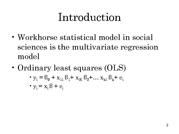Introduction • Workhorse statistical model in social sciences is the multivariate regression model • Ordinary least squares (OLS) • yi = β 0 + x 1 i β 1+ x 2 i β 2+… xki βk+ εi • yi = x i β + ε i 2

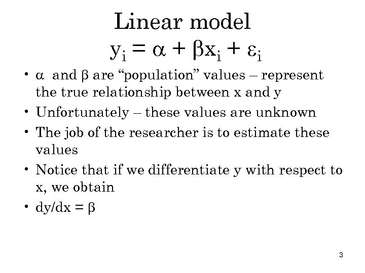Linear model yi = + xi + i • and are “population” values – represent the true relationship between x and y • Unfortunately – these values are unknown • The job of the researcher is to estimate these values • Notice that if we differentiate y with respect to x, we obtain • dy/dx = 3

• represents how much y will change for a fixed change in x – Increase in income for more education – Change in crime or bankruptcy when slots are legalized – Increase in test score if you study more 4

Put some concreteness on the problem • State of Maryland budget problems – Drop in revenues – Expensive k-12 school spending initiatives • Short-term solution – raise tax on cigarettes by 34 cents/pack • Problem – a tax hike will reduce consumption of taxable product • Question for state – as taxes are raised, how much will cigarette consumption fall? 5

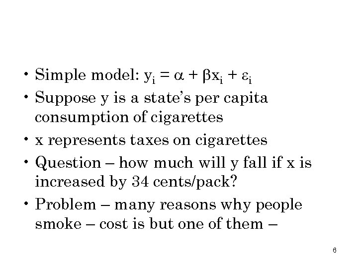• Simple model: yi = + xi + i • Suppose y is a state’s per capita consumption of cigarettes • x represents taxes on cigarettes • Question – how much will y fall if x is increased by 34 cents/pack? • Problem – many reasons why people smoke – cost is but one of them – 6

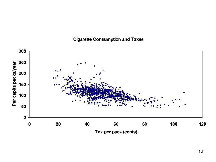
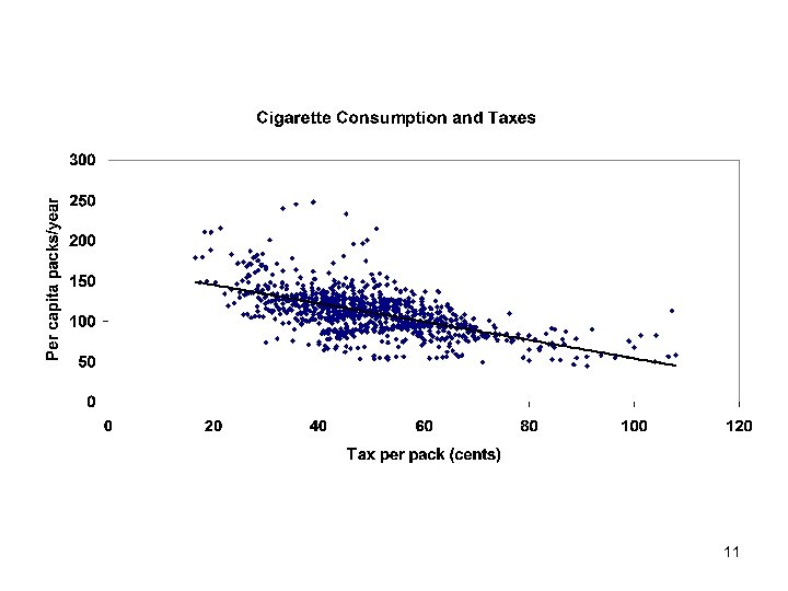
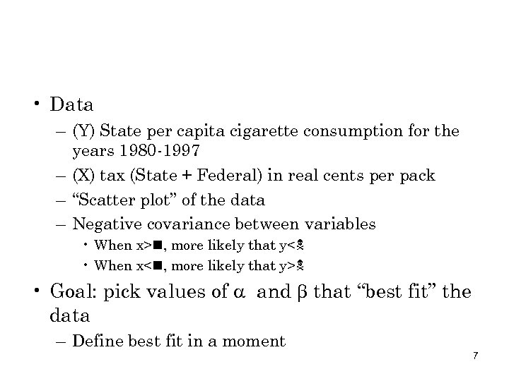• Data – (Y) State per capita cigarette consumption for the years 1980 -1997 – (X) tax (State + Federal) in real cents per pack – “Scatter plot” of the data – Negative covariance between variables • When x> , more likely that y< • When x< , more likely that y> • Goal: pick values of and that “best fit” the data – Define best fit in a moment 7

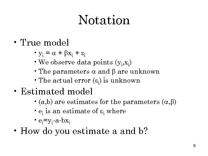Notation • True model • yi = + xi + i • We observe data points (yi, xi) • The parameters and are unknown • The actual error ( i) is unknown • Estimated model • (a, b) are estimates for the parameters ( , ) • ei is an estimate of i where • ei=yi-a-bxi • How do you estimate a and b? 8

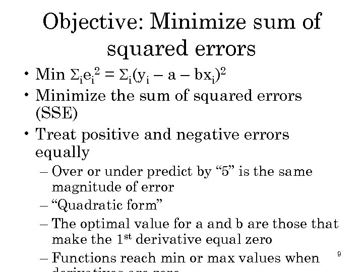Objective: Minimize sum of squared errors • Min iei 2 = i(yi – a – bxi)2 • Minimize the sum of squared errors (SSE) • Treat positive and negative errors equally – Over or under predict by “ 5” is the same magnitude of error – “Quadratic form” – The optimal value for a and b are those that make the 1 st derivative equal zero – Functions reach min or max values when 9

10

11

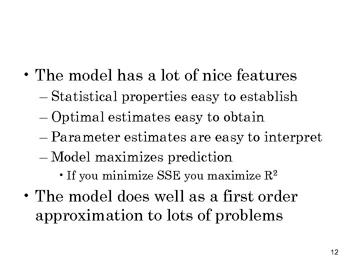• The model has a lot of nice features – Statistical properties easy to establish – Optimal estimates easy to obtain – Parameter estimates are easy to interpret – Model maximizes prediction • If you minimize SSE you maximize R 2 • The model does well as a first order approximation to lots of problems 12

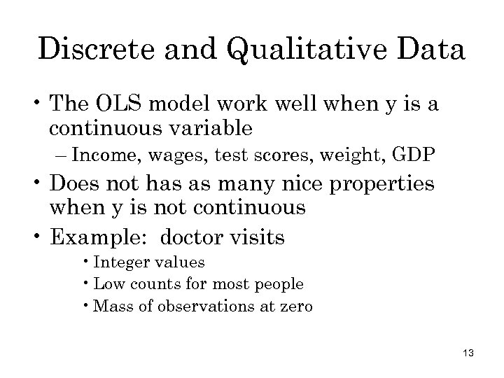Discrete and Qualitative Data • The OLS model work well when y is a continuous variable – Income, wages, test scores, weight, GDP • Does not has as many nice properties when y is not continuous • Example: doctor visits • Integer values • Low counts for most people • Mass of observations at zero 13

Downside of forcing non-standard outcomes into OLS world? • Can predict outside the allowable range – e. g. , negative MD visits • Does not describe the data generating process well – e. g. , mass of observations at zero • Violates many properties of OLS – e. g. heteroskedasticity 14

This talk • Look at situations when the data generating process does lend itself well to OLS models • Mathematically describe the data generating process • Show we use different optimization procedure to obtain estimates • Describe the statistical properties 15

• Show to interpret parameters • Illustrate how to estimate the models with popular program STATA 16

Types of data generating processes we will consider • Dichotomous events (yes or no) – 1=yes, 0=no – Graduate high school? work? Are obese? Smoke? • Ordinal data – Self reported health (fair, poor, good, excel) – Strongly disagree, strongly agree 17

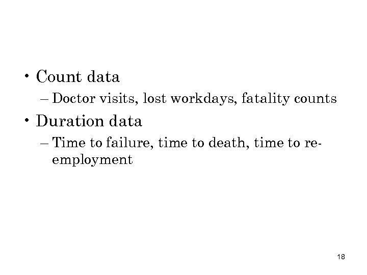• Count data – Doctor visits, lost workdays, fatality counts • Duration data – Time to failure, time to death, time to reemployment 18

Econometric Resources • Recommended textbook – Jeffrey Wooldridge, undergraduate and grad – Lots of insight and mathematical/statistical detail – Very good examples • Helpful web sites – My graduate class – Jeff Smith’s class 19

STATA • Very fast, convenient, well-documented, cheap and flexible statistical package • Excellent for cross-section/panel data projects, not as great for time series • Not as easy to manipulate large data sets from flat files as SAS • I usually clean data in SAS, estimate models in STATA 20

STATA Resources - Specific • “Regression Models for Categorical Dependent Variables Using STATA” – J. Scott Long and Jeremy Freese • Available for sale from STATA website for $52 (www. stata. com) • Post-estimation subroutines that translate results – Do not need to buy the book to use the subroutines 21

• In STATA command line type • net search spost • Will give you a list of available programs to download • One is Spostado from http: //www. indiana. edu/~jslsoc/stata • Click on the link and install the files 22

Continuous Distributions • Random variables with infinite number of possible values • Examples -- units of measure (time, weight, distance) • Many discrete outcomes can be treated as continuous, e. g. , SAT scores 23

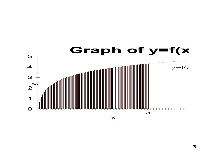
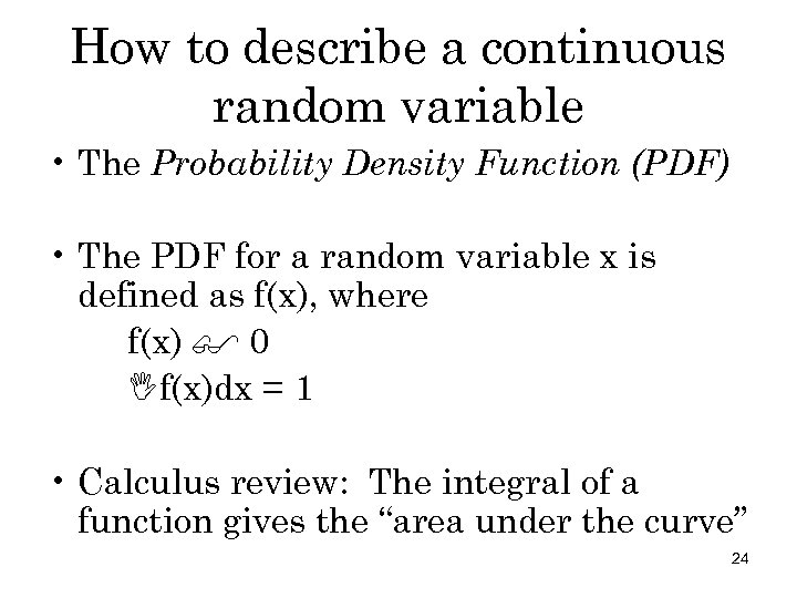How to describe a continuous random variable • The Probability Density Function (PDF) • The PDF for a random variable x is defined as f(x), where f(x) $ 0 If(x)dx = 1 • Calculus review: The integral of a function gives the “area under the curve” 24

25

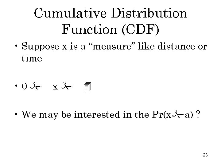Cumulative Distribution Function (CDF) • Suppose x is a “measure” like distance or time • 0 x • We may be interested in the Pr(x a) ? 26

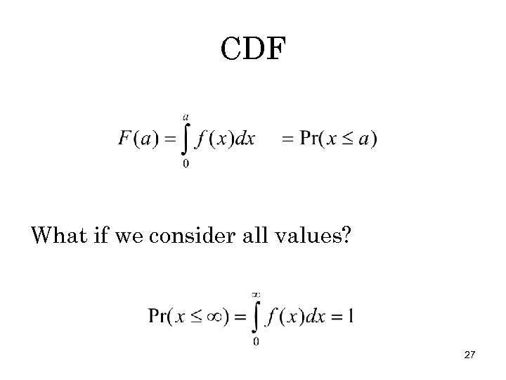CDF What if we consider all values? 27

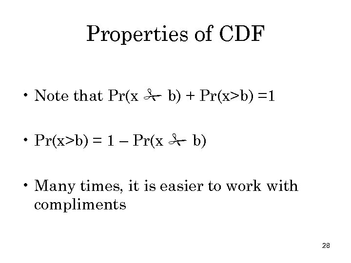Properties of CDF • Note that Pr(x b) + Pr(x>b) =1 • Pr(x>b) = 1 – Pr(x b) • Many times, it is easier to work with compliments 28

General notation for continuous distributions • The PDF is described by lower case such as f(x) • The CDF is defined as upper case such as F(a) 29

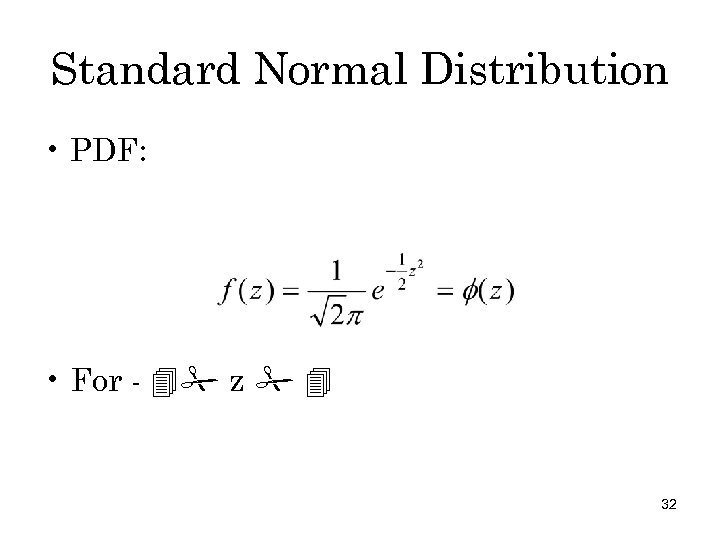
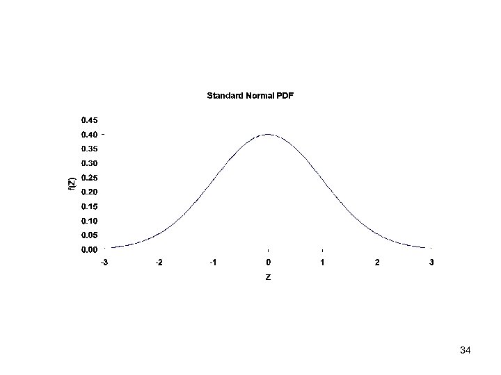
Standard Normal Distribution • Most frequently used continuous distribution • Symmetric “bell-shaped” distribution • As we will show, the normal has useful properties • Many variables we observe in the real world look normally distributed. • Can translate normal into ‘standard normal’ 30

Examples of variables that look normally distributed • IQ scores • SAT scores • Heights of females • Log income • Average gestation (weeks of pregnancy) • As we will show in a few weeks – sample means are normally distributed!!! 31

Standard Normal Distribution • PDF: • For - z 32

Notation • (z) is the standard normal PDF evaluated at z • [a] = Pr(z a) 33

34

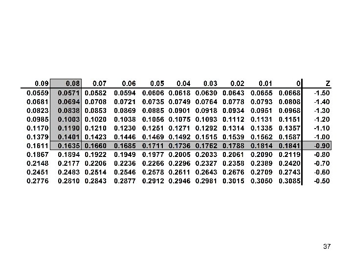
Standard Normal • Notice that: – – – Normal is symmetric: (a) = (-a) Normal is “unimodal” Median=mean Area under curve=1 Almost all area is between (-3, 3) • Evaluations of the CDF are done with – Statistical functions (excel, SAS, etc) – Tables 35

Standard Normal CDF • Pr(z -0. 98) = [-0. 98] = 0. 1635 36

37

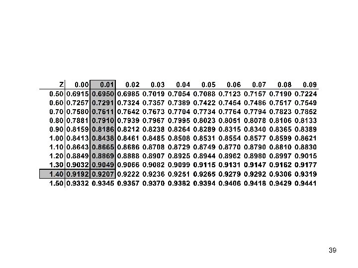
• Pr(z 1. 41) = [1. 41] = 0. 9207 38

39

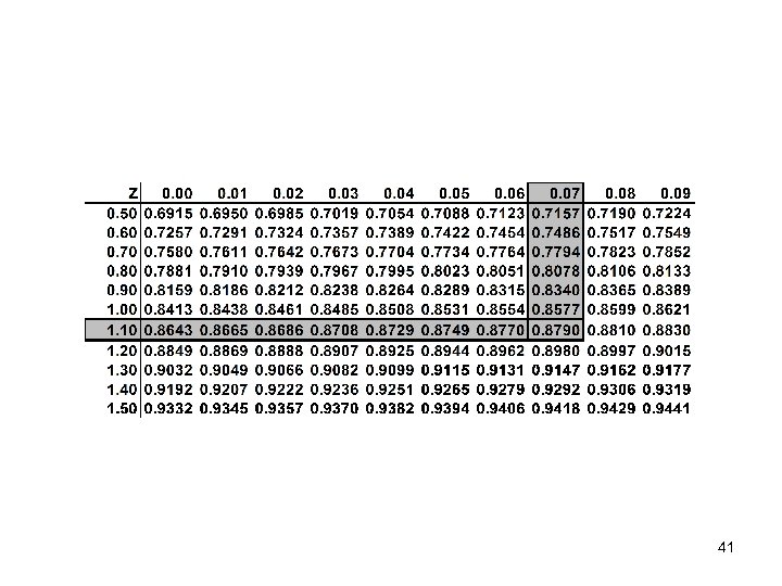
• Pr(x>1. 17) = 1 – Pr(z 1. 17) = 1 [1. 17] • = 1 – 0. 8790 = 0. 1210 40

41

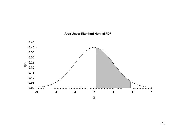
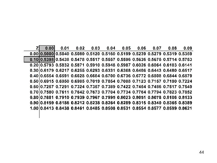
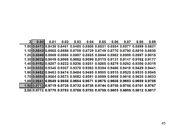
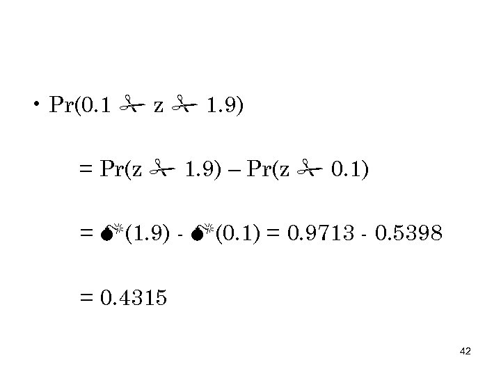• Pr(0. 1 z 1. 9) = Pr(z 1. 9) – Pr(z 0. 1) = (1. 9) - (0. 1) = 0. 9713 - 0. 5398 = 0. 4315 42

43

44

45

Important Properties of Normal Distribution • Pr(z A) = [A] • Pr(z > A) = 1 - [A] • Pr(z - A) = [-A] • Pr(z > -A) = 1 - [-A] = [A] 46

Maximum likelihood estimation • Observe n independent outcomes, all drawn from the same distribution • (y 1, y 2, y 3…. yn) • yi is drawn from f(yi; θ) where θ is an unknown parameter for the distribution f • Recall definition of indepedence. If a and b and independent, Prob(a and b) = Pr(a)Pr(B) 47

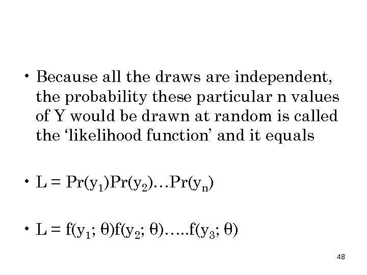• Because all the draws are independent, the probability these particular n values of Y would be drawn at random is called the ‘likelihood function’ and it equals • L = Pr(y 1)Pr(y 2)…Pr(yn) • L = f(y 1; θ)f(y 2; θ)…. . f(y 3; θ) 48

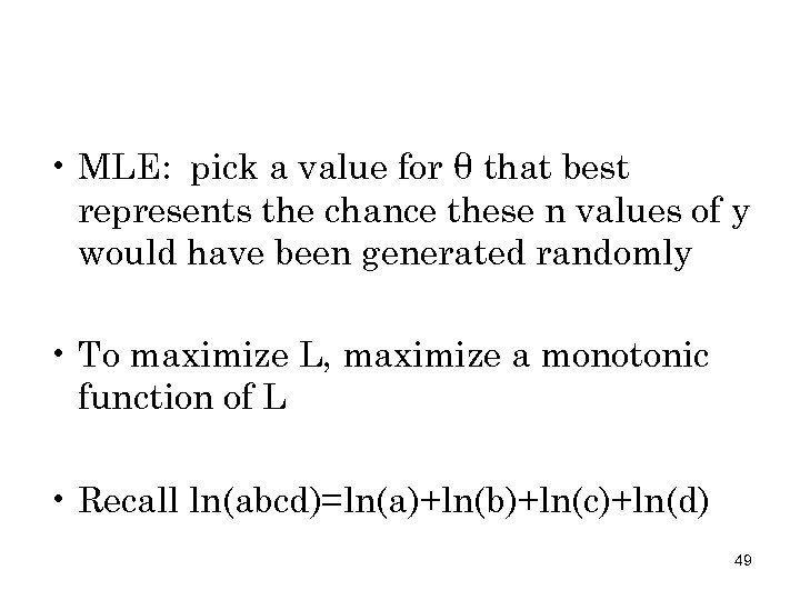• MLE: pick a value for θ that best represents the chance these n values of y would have been generated randomly • To maximize L, maximize a monotonic function of L • Recall ln(abcd)=ln(a)+ln(b)+ln(c)+ln(d) 49

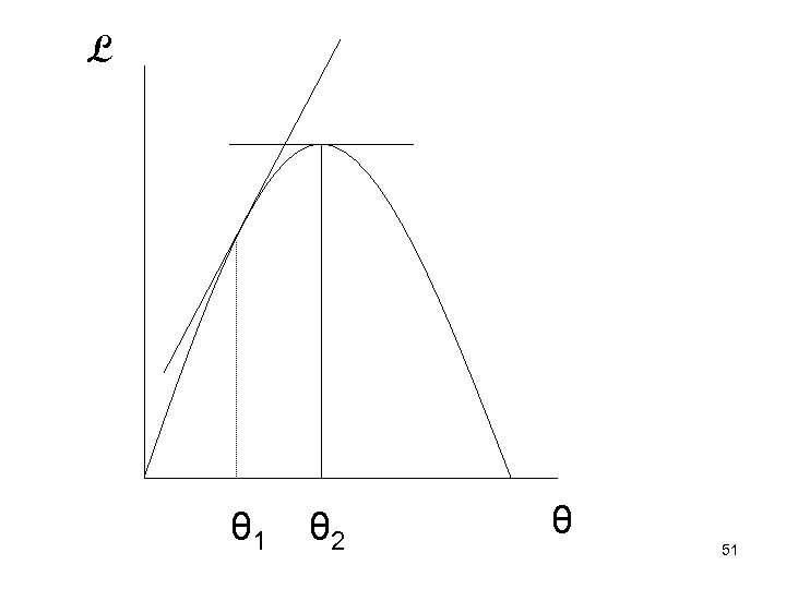
• Max L = ln(L) = ln[f(y 1; θ)] +ln[f(y 2; θ)] + …. . ln[f(yn; θ) = Σi ln[f(yi; θ)] • Pick θ so that L is maximized • d. L/dθ = 0 50

L θ 1 θ 2 θ 51

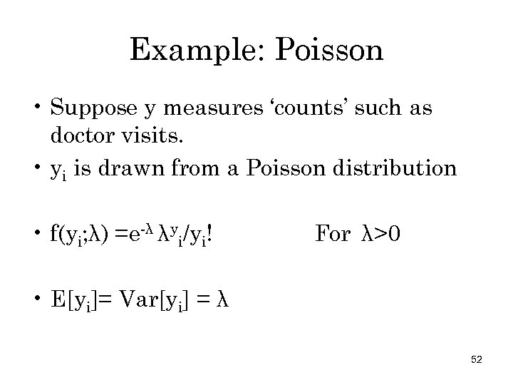Example: Poisson • Suppose y measures ‘counts’ such as doctor visits. • yi is drawn from a Poisson distribution • f(yi; λ) =e-λ λyi/yi! For λ>0 • E[yi]= Var[yi] = λ 52

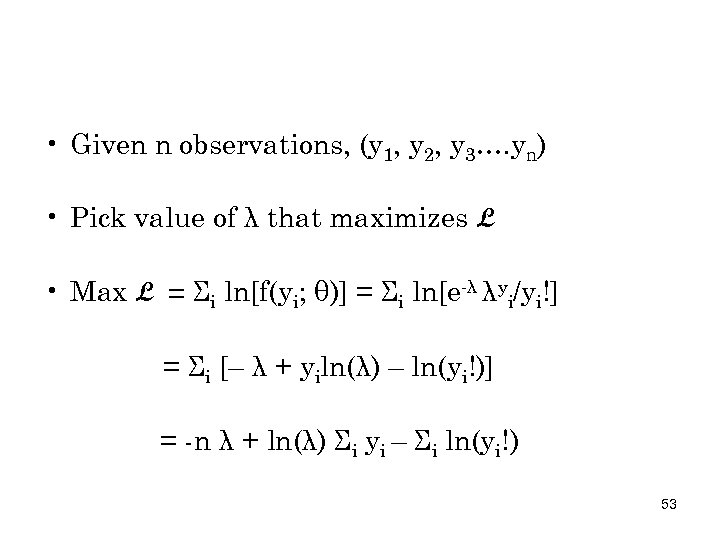• Given n observations, (y 1, y 2, y 3…. yn) • Pick value of λ that maximizes L • Max L = Σi ln[f(yi; θ)] = Σi ln[e-λ λyi/yi!] = Σi [– λ + yiln(λ) – ln(yi!)] = -n λ + ln(λ) Σi yi – Σi ln(yi!) 53

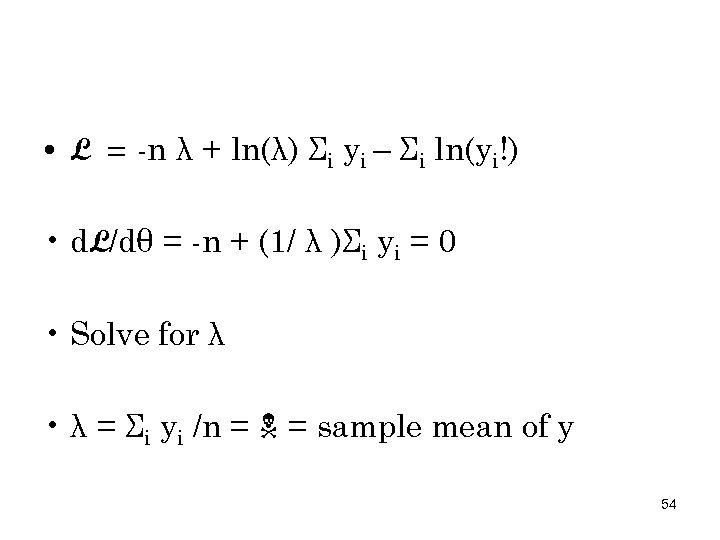• L = -n λ + ln(λ) Σi yi – Σi ln(yi!) • d. L/dθ = -n + (1/ λ )Σi yi = 0 • Solve for λ • λ = Σi yi /n = = sample mean of y 54

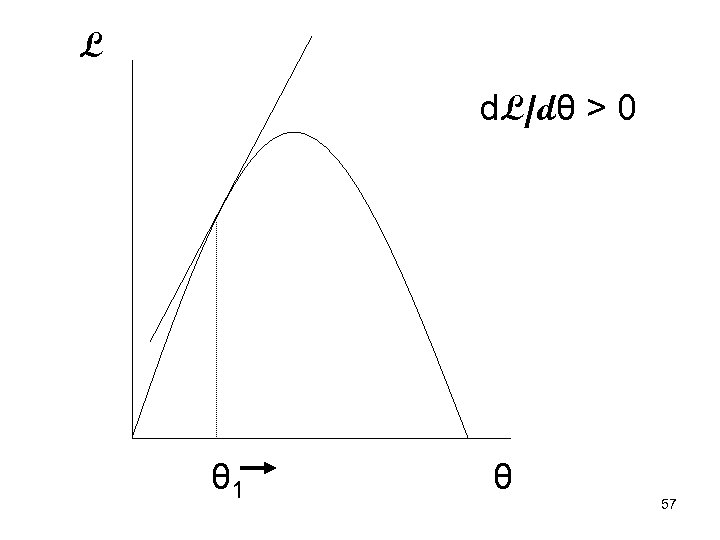
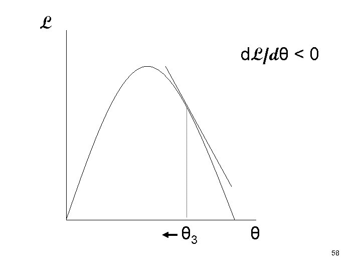
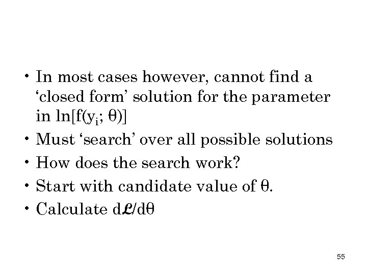• In most cases however, cannot find a ‘closed form’ solution for the parameter in ln[f(yi; θ)] • Must ‘search’ over all possible solutions • How does the search work? • Start with candidate value of θ. • Calculate d. L/dθ 55

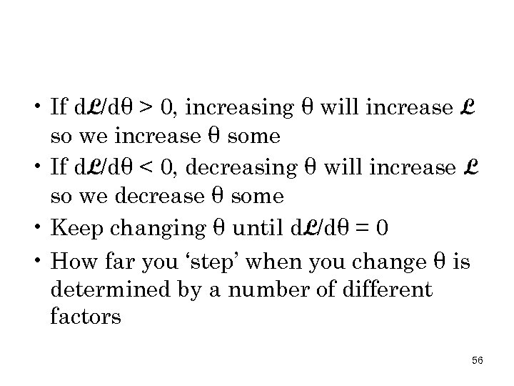• If d. L/dθ > 0, increasing θ will increase L so we increase θ some • If d. L/dθ < 0, decreasing θ will increase L so we decrease θ some • Keep changing θ until d. L/dθ = 0 • How far you ‘step’ when you change θ is determined by a number of different factors 56

L d. L/dθ > 0 θ 1 θ 57

L d. L/dθ < 0 θ 3 θ 58

Properties of MLE estimates • Sometimes call efficient estimation. Can never generate a smaller variance than one obtained by MLE • Parameters estimates are distributed as a normal distribution when samples sizes are large 59