b5707b29eab4372fb8188e5c594f81dd.ppt
- Количество слайдов: 174
 Digital Image Processing: 1
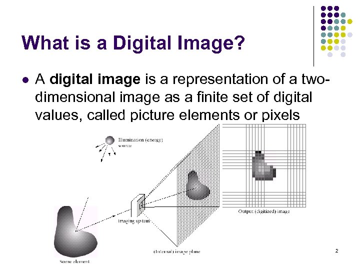 What is a Digital Image? l A digital image is a representation of a twodimensional image as a finite set of digital values, called picture elements or pixels 2
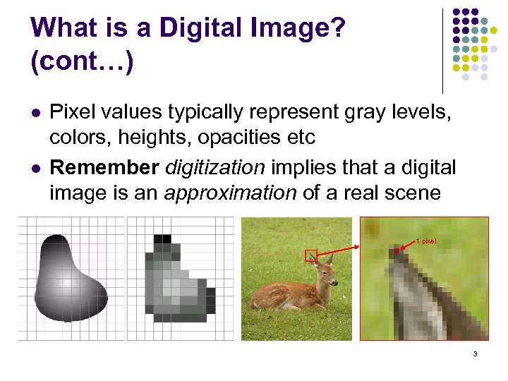 What is a Digital Image? (cont…) l l Pixel values typically represent gray levels, colors, heights, opacities etc Remember digitization implies that a digital image is an approximation of a real scene 1 pixel 3
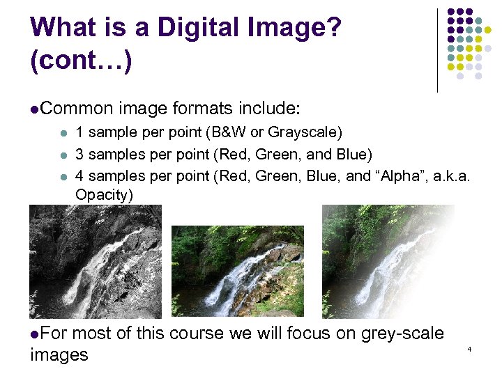 What is a Digital Image? (cont…) l. Common l l l image formats include: 1 sample per point (B&W or Grayscale) 3 samples per point (Red, Green, and Blue) 4 samples per point (Red, Green, Blue, and “Alpha”, a. k. a. Opacity) l. For most of this course we will focus on grey-scale images 4
 What is Digital Image Processing? l Digital image processing focuses on two major tasks l l l Improvement of pictorial information for human interpretation Processing of image data for storage, transmission and representation for autonomous machine perception Some argument about where image processing ends and fields such as image analysis and computer vision start 5
 What is DIP? (cont…) l The continuum from image processing to computer vision can be broken up into low-, mid- and high-level processes Low Level Process Mid Level Process High Level Process Input: Image Output: Image Input: Image Output: Attributes Input: Attributes Output: Understanding Examples: Noise removal, image sharpening Examples: Object recognition, segmentation Examples: Scene understanding, autonomous navigation In this course we will stop here 6
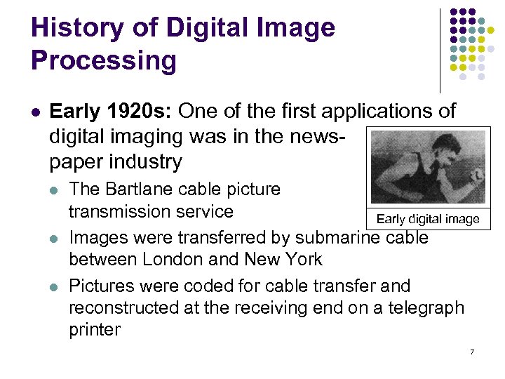 History of Digital Image Processing l Early 1920 s: One of the first applications of digital imaging was in the newspaper industry l l l The Bartlane cable picture transmission service Early digital image Images were transferred by submarine cable between London and New York Pictures were coded for cable transfer and reconstructed at the receiving end on a telegraph printer 7
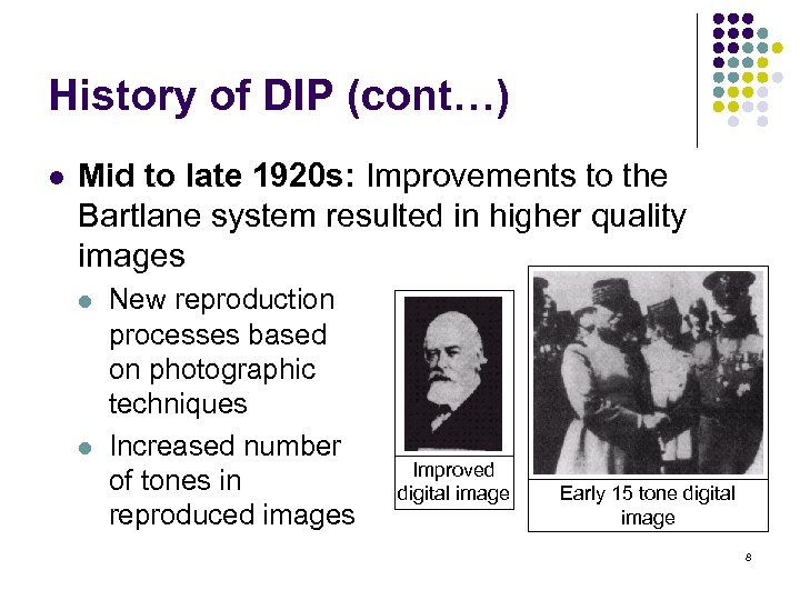 History of DIP (cont…) l Mid to late 1920 s: Improvements to the Bartlane system resulted in higher quality images l l New reproduction processes based on photographic techniques Increased number of tones in reproduced images Improved digital image Early 15 tone digital image 8
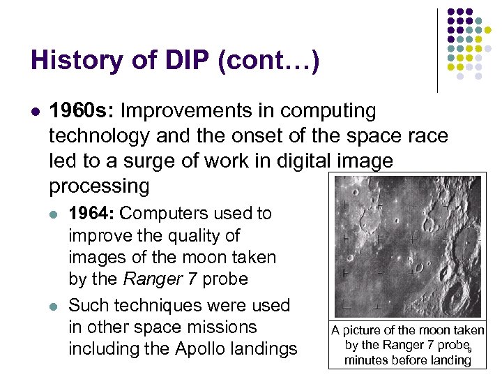 History of DIP (cont…) l 1960 s: Improvements in computing technology and the onset of the space race led to a surge of work in digital image processing l l 1964: Computers used to improve the quality of images of the moon taken by the Ranger 7 probe Such techniques were used in other space missions including the Apollo landings A picture of the moon taken by the Ranger 7 probe 9 minutes before landing
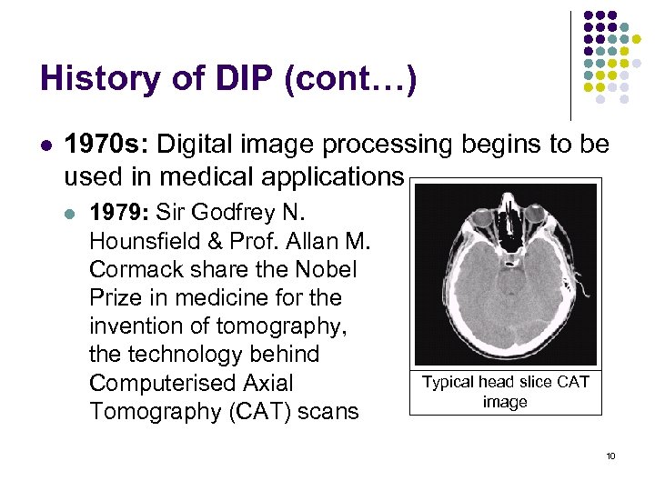 History of DIP (cont…) l 1970 s: Digital image processing begins to be used in medical applications l 1979: Sir Godfrey N. Hounsfield & Prof. Allan M. Cormack share the Nobel Prize in medicine for the invention of tomography, the technology behind Computerised Axial Tomography (CAT) scans Typical head slice CAT image 10
 History of DIP (cont…) l 1980 s - Today: The use of digital image processing techniques has exploded and they are now used for all kinds of tasks in all kinds of areas l l l Image enhancement/restoration Artistic effects Medical visualisation Industrial inspection Law enforcement Human computer interfaces 11
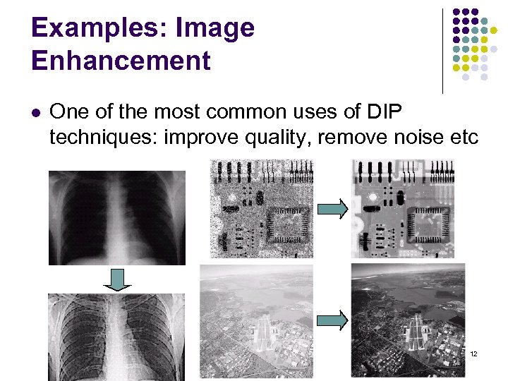 Examples: Image Enhancement l One of the most common uses of DIP techniques: improve quality, remove noise etc 12
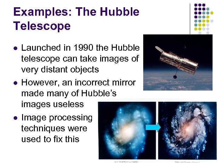 Examples: The Hubble Telescope l l l Launched in 1990 the Hubble telescope can take images of very distant objects However, an incorrect mirror made many of Hubble’s images useless Image processing techniques were used to fix this 13
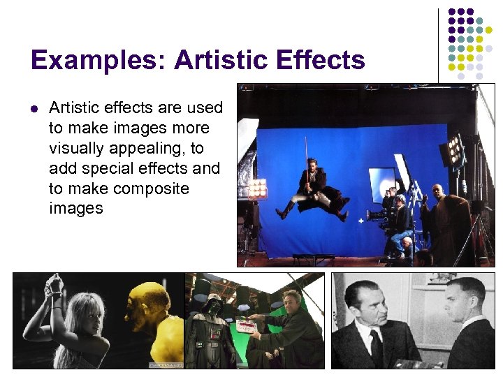 Examples: Artistic Effects l Artistic effects are used to make images more visually appealing, to add special effects and to make composite images 14
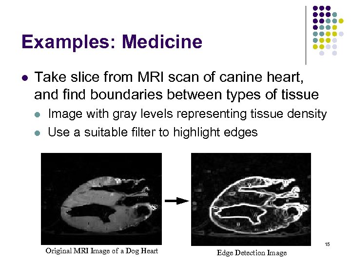 Examples: Medicine l Take slice from MRI scan of canine heart, and find boundaries between types of tissue l l Image with gray levels representing tissue density Use a suitable filter to highlight edges Original MRI Image of a Dog Heart 15 Edge Detection Image
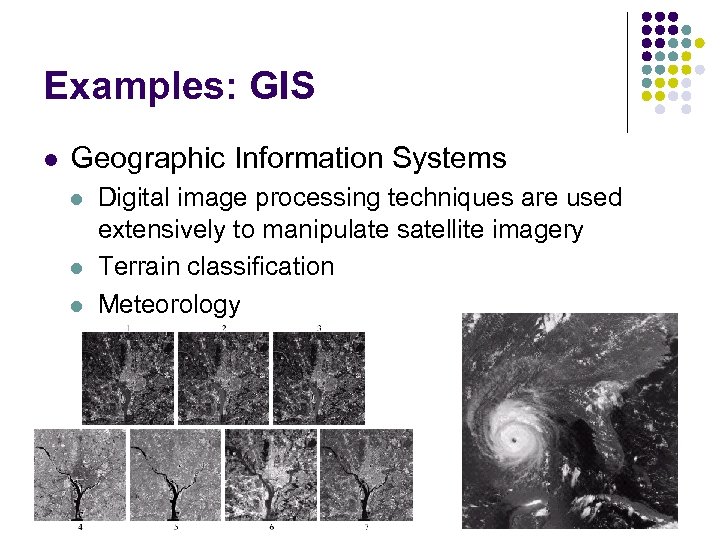 Examples: GIS l Geographic Information Systems l l l Digital image processing techniques are used extensively to manipulate satellite imagery Terrain classification Meteorology 16
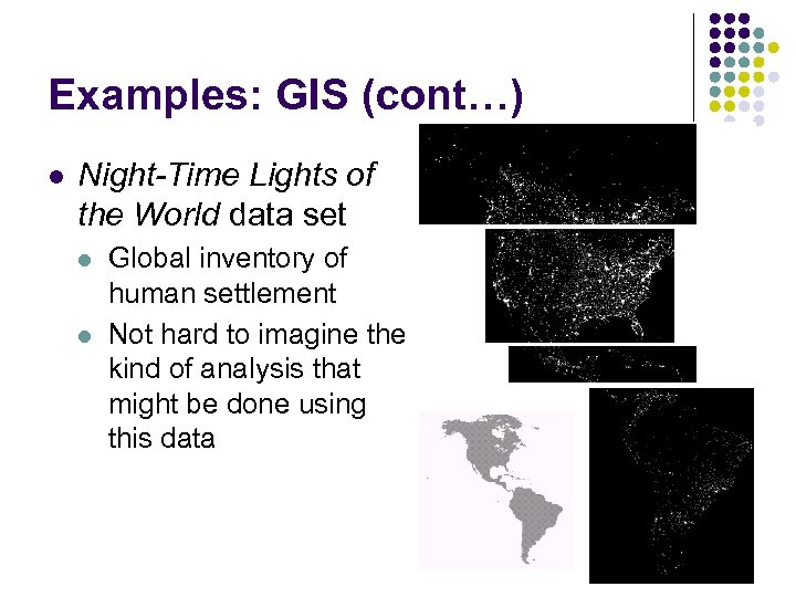 Examples: GIS (cont…) l Night-Time Lights of the World data set l l Global inventory of human settlement Not hard to imagine the kind of analysis that might be done using this data 17
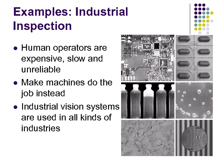 Examples: Industrial Inspection l l l Human operators are expensive, slow and unreliable Make machines do the job instead Industrial vision systems are used in all kinds of industries 18
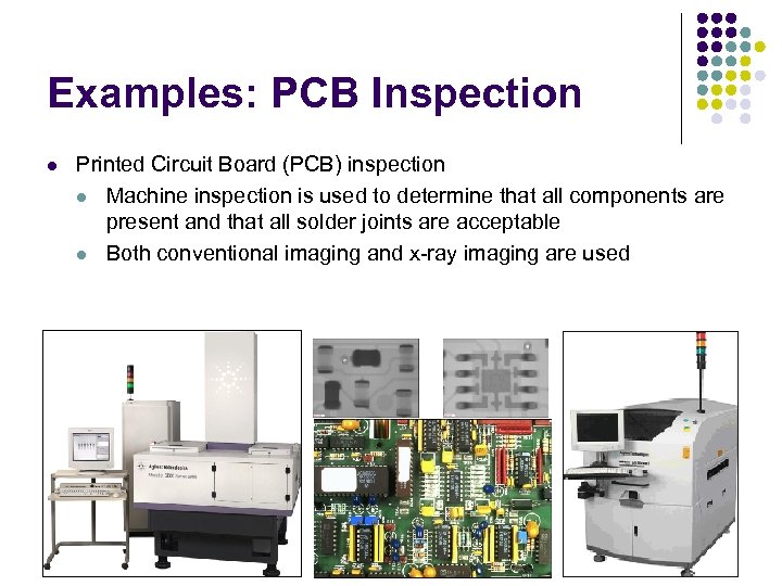 Examples: PCB Inspection l Printed Circuit Board (PCB) inspection l Machine inspection is used to determine that all components are present and that all solder joints are acceptable l Both conventional imaging and x-ray imaging are used 19
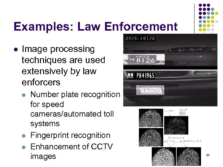 Examples: Law Enforcement l Image processing techniques are used extensively by law enforcers l l l Number plate recognition for speed cameras/automated toll systems Fingerprint recognition Enhancement of CCTV images 20
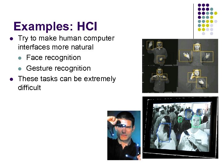 Examples: HCI l l Try to make human computer interfaces more natural l Face recognition l Gesture recognition These tasks can be extremely difficult 21
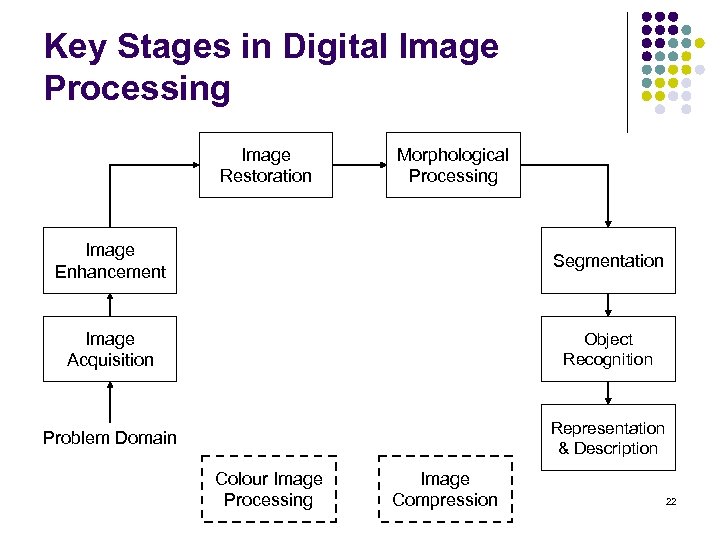 Key Stages in Digital Image Processing Image Restoration Morphological Processing Image Enhancement Segmentation Image Acquisition Object Recognition Problem Domain Representation & Description Colour Image Processing Image Compression 22
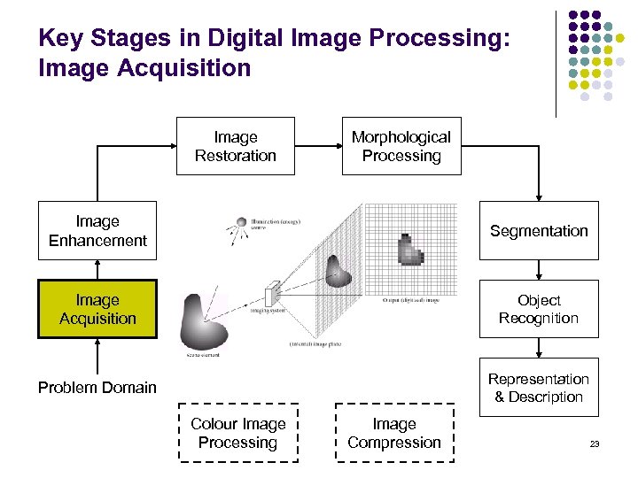 Key Stages in Digital Image Processing: Image Acquisition Image Restoration Morphological Processing Image Enhancement Segmentation Image Acquisition Object Recognition Problem Domain Representation & Description Colour Image Processing Image Compression 23
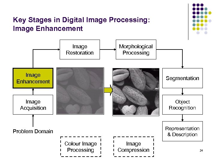 Key Stages in Digital Image Processing: Image Enhancement Image Restoration Morphological Processing Image Enhancement Segmentation Image Acquisition Object Recognition Problem Domain Representation & Description Colour Image Processing Image Compression 24
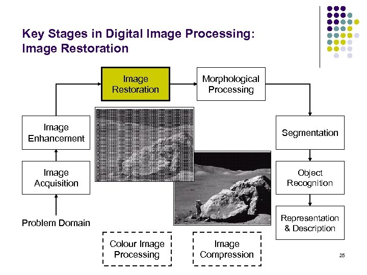 Key Stages in Digital Image Processing: Image Restoration Morphological Processing Image Enhancement Segmentation Image Acquisition Object Recognition Problem Domain Representation & Description Colour Image Processing Image Compression 25
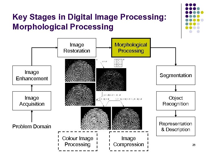 Key Stages in Digital Image Processing: Morphological Processing Image Restoration Morphological Processing Image Enhancement Segmentation Image Acquisition Object Recognition Problem Domain Representation & Description Colour Image Processing Image Compression 26
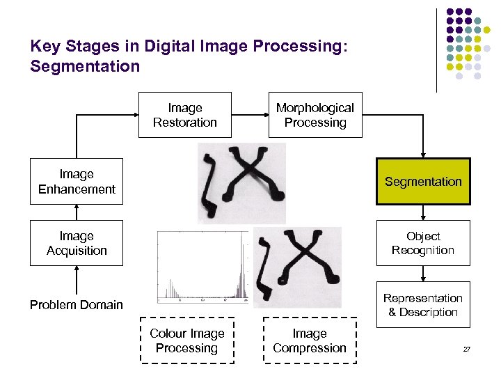 Key Stages in Digital Image Processing: Segmentation Image Restoration Morphological Processing Image Enhancement Segmentation Image Acquisition Object Recognition Problem Domain Representation & Description Colour Image Processing Image Compression 27
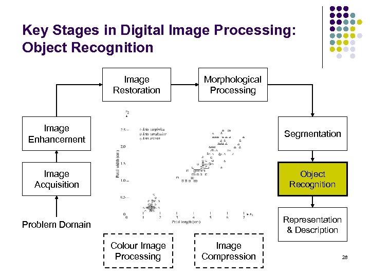 Key Stages in Digital Image Processing: Object Recognition Image Restoration Morphological Processing Image Enhancement Segmentation Image Acquisition Object Recognition Problem Domain Representation & Description Colour Image Processing Image Compression 28
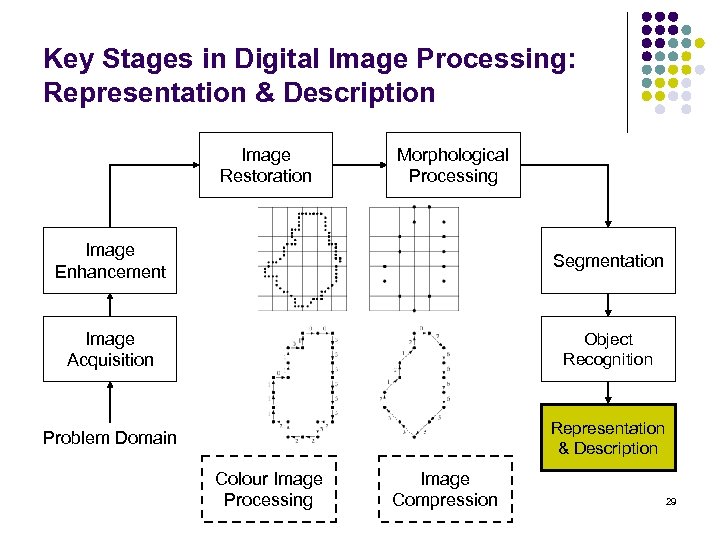 Key Stages in Digital Image Processing: Representation & Description Image Restoration Morphological Processing Image Enhancement Segmentation Image Acquisition Object Recognition Problem Domain Representation & Description Colour Image Processing Image Compression 29
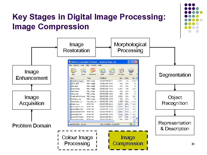 Key Stages in Digital Image Processing: Image Compression Image Restoration Morphological Processing Image Enhancement Segmentation Image Acquisition Object Recognition Problem Domain Representation & Description Colour Image Processing Image Compression 30
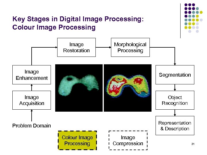 Key Stages in Digital Image Processing: Colour Image Processing Image Restoration Morphological Processing Image Enhancement Segmentation Image Acquisition Object Recognition Problem Domain Representation & Description Colour Image Processing Image Compression 31
 CONTINUOUS IMAGE MATHEMATICAL CHARACTERIZATION There are two basic mathematical characterizations of interest: deterministic and statistical. l In deterministic image representation, a mathematical image function is defined and point properties of the image are considered. l For a statistical image representation, the image is specified by average properties. l 32
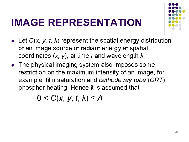 IMAGE REPRESENTATION l l Let C(x, y, t, λ) represent the spatial energy distribution of an image source of radiant energy at spatial coordinates (x, y), at time t and wavelength λ. The physical imaging system also imposes some restriction on the maximum intensity of an image, for example, film saturation and cathode ray tube (CRT) phosphor heating. Hence it is assumed that 0 < C(x, y, t, λ) ≤ A 33
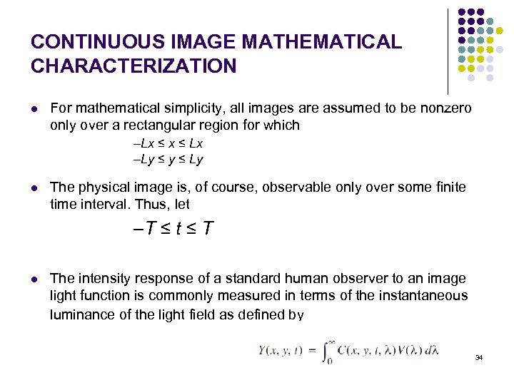 CONTINUOUS IMAGE MATHEMATICAL CHARACTERIZATION l For mathematical simplicity, all images are assumed to be nonzero only over a rectangular region for which –Lx ≤ Lx –Ly ≤ Ly l The physical image is, of course, observable only over some finite time interval. Thus, let –T ≤ t ≤ T l The intensity response of a standard human observer to an image light function is commonly measured in terms of the instantaneous luminance of the light field as defined by 34
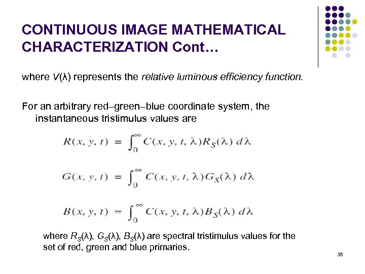 CONTINUOUS IMAGE MATHEMATICAL CHARACTERIZATION Cont… where V(λ) represents the relative luminous efficiency function. For an arbitrary red–green–blue coordinate system, the instantaneous tristimulus values are where RS(λ), GS(λ), BS(λ) are spectral tristimulus values for the set of red, green and blue primaries. 35
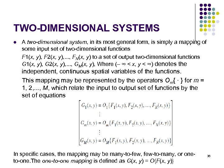 TWO-DIMENSIONAL SYSTEMS l A two-dimensional system, in its most general form, is simply a mapping of some input set of two-dimensional functions F 1(x, y), F 2(x, y), . . . , FN(x, y) to a set of output two-dimensional functions G 1(x, y), G 2(x, y), . . . , GM(x, y), Where (– ∞ < x, y < ∞) denotes the independent, continuous spatial variables of the functions. This mapping may be represented by the operators Om{ · } for m = 1, 2, . . . , M, which relate the input to output set of functions by the set of equations In specific cases, the mapping may be many-to-few, few-to-many, or oneto-one. The one-to-one mapping is defined as G(x, y) = O{F(x, y)} 36
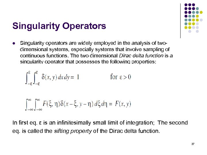 Singularity Operators l Singularity operators are widely employed in the analysis of twodimensional systems, especially systems that involve sampling of continuous functions. The two dimensional Dirac delta function is a singularity operator that possesses the following properties: In first eq. ε is an infinitesimally small limit of integration; The second eq. is called the sifting property of the Dirac delta function. 37
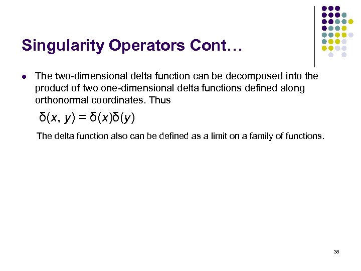 Singularity Operators Cont… l The two-dimensional delta function can be decomposed into the product of two one-dimensional delta functions defined along orthonormal coordinates. Thus δ(x, y) = δ(x)δ(y) The delta function also can be defined as a limit on a family of functions. 38
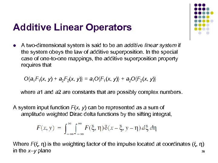 Additive Linear Operators l A two-dimensional system is said to be an additive linear system if the system obeys the law of additive superposition. In the special case of one-to-one mappings, the additive superposition property requires that O{a 1 F 1(x, y) + a 2 F 2(x, y)} = a 1 O{F 1(x, y)} + a 2 O{F 2(x, y)} where a 1 and a 2 are constants that are possibly complex numbers. A system input function F(x, y) can be represented as a sum of amplitude weighted Dirac delta functions by the sifting integral, Where F(ξ, η) is the weighting factor of the impulse located at coordinates (ξ, η) in the x–y plane 39
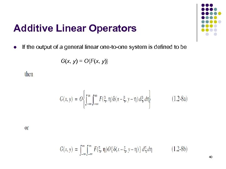 Additive Linear Operators l If the output of a general linear one-to-one system is defined to be G(x, y) = O{F(x, y)} 40
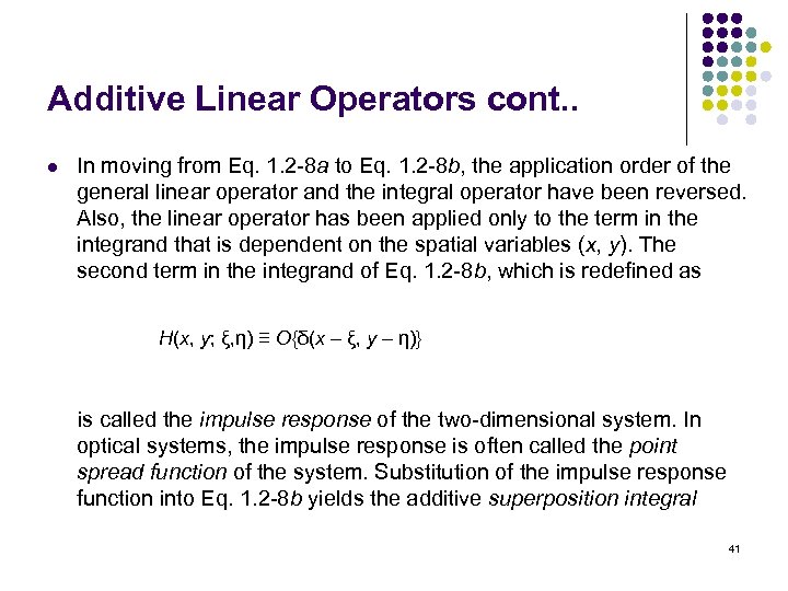 Additive Linear Operators cont. . l In moving from Eq. 1. 2 -8 a to Eq. 1. 2 -8 b, the application order of the general linear operator and the integral operator have been reversed. Also, the linear operator has been applied only to the term in the integrand that is dependent on the spatial variables (x, y). The second term in the integrand of Eq. 1. 2 -8 b, which is redefined as H(x, y; ξ, η) ≡ O{δ(x – ξ, y – η)} is called the impulse response of the two-dimensional system. In optical systems, the impulse response is often called the point spread function of the system. Substitution of the impulse response function into Eq. 1. 2 -8 b yields the additive superposition integral 41
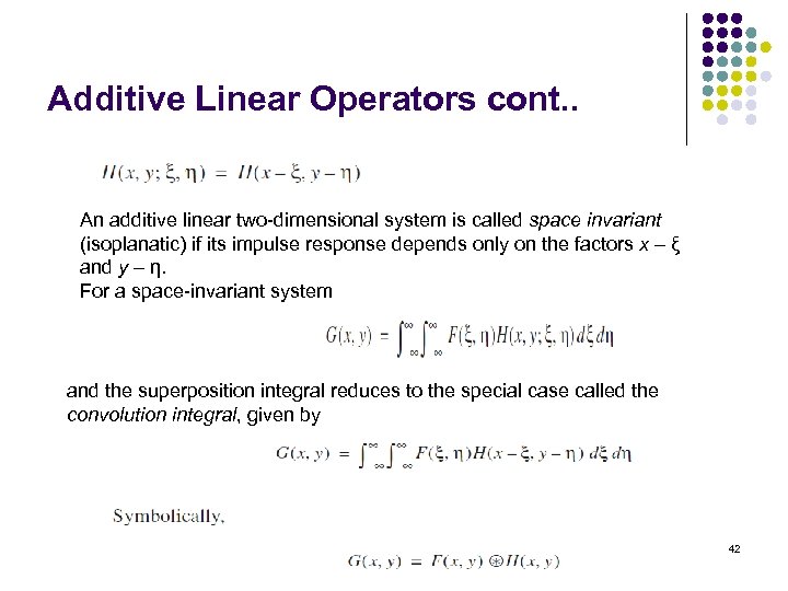 Additive Linear Operators cont. . An additive linear two-dimensional system is called space invariant (isoplanatic) if its impulse response depends only on the factors x – ξ and y – η. For a space-invariant system and the superposition integral reduces to the special case called the convolution integral, given by 42
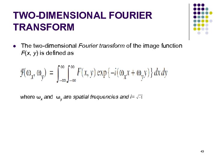 TWO-DIMENSIONAL FOURIER TRANSFORM l The two-dimensional Fourier transform of the image function F(x, y) is defined as where ωx and ωy are spatial frequencies and i= 43
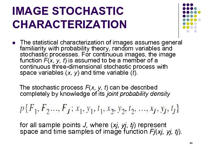 IMAGE STOCHASTIC CHARACTERIZATION l The statistical characterization of images assumes general familiarity with probability theory, random variables and stochastic processes. For continuous images, the image function F(x, y, t) is assumed to be a member of a continuous three-dimensional stochastic process with space variables (x, y) and time variable (t). The stochastic process F(x, y, t) can be described completely by knowledge of its joint probability density for all sample points J, where (xj, yj, tj) represent space and time samples of image function Fj(xj, yj, tj). 44
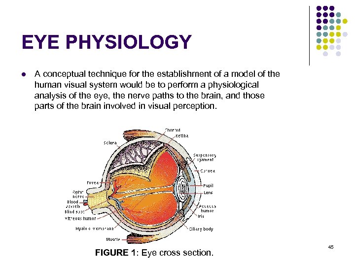 EYE PHYSIOLOGY l A conceptual technique for the establishment of a model of the human visual system would be to perform a physiological analysis of the eye, the nerve paths to the brain, and those parts of the brain involved in visual perception. FIGURE 1: Eye cross section. 45
 EYE PHYSIOLOGY Figure 1 shows the horizontal cross section of a human eyeball. The front of the eye is covered by a transparent surface called the cornea. The remaining outer cover, called the sclera, is composed of a fibrous coat that surrounds the choroid, a layer containing blood capillaries. Inside the choroid is the retina, which is composed of two types of receptors: rods and cones. Nerves connecting to the retina leave the eyeball through the optic nerve bundle. Light entering the cornea is focused on the retina surface by a lens that changes shape under muscular control to perform proper focusing of near and distant objects. An iris acts as a diaphram to control the amount of light entering the eye. 46
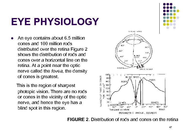 EYE PHYSIOLOGY l An eye contains about 6. 5 million cones and 100 million rods distributed over the retina Figure 2 shows the distribution of rods and cones over a horizontal line on the retina. At a point near the optic nerve called the fovea, the density of cones is greatest. This is the region of sharpest photopic vision. There are no rods or cones in the vicinity of the optic nerve, and hence the eye has a blind spot in this region. FIGURE 2. Distribution of rods and cones on the retina 47
 Visual Perception: Human Eye 1. The lens contains 60 -70% water, 6% of fat. 2. 3. The iris diaphragm controls amount of light that enters the eye. Light receptors in the retina - About 6 -7 millions cones for bright light vision called photopic - Density of cones is about 150, 000 elements/mm 2. 1. - Cones involve in color vision. 2. - Cones are concentrated in fovea about 1. 5 x 1. 5 mm 2. 3. - About 75 -150 millions rods for dim light vision called scotopic 4. - Rods are sensitive to low level of light and are not involved 5. color vision. 4. Blind spot is the region of emergence of the optic nerve from the eye. 48
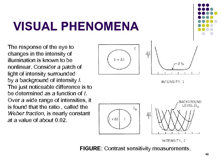 VISUAL PHENOMENA The response of the eye to changes in the intensity of illumination is known to be nonlinear. Consider a patch of light of intensity surrounded by a background of intensity I. The just noticeable difference is to be determined as a function of I. Over a wide range of intensities, it is found that the ratio , called the Weber fraction, is nearly constant at a value of about 0. 02. FIGURE: Contrast sensitivity measurements. 49
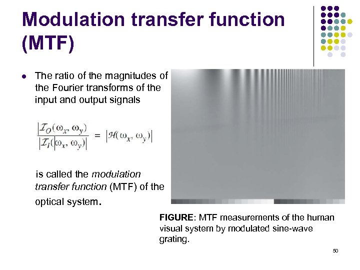 Modulation transfer function (MTF) l The ratio of the magnitudes of the Fourier transforms of the input and output signals is called the modulation transfer function (MTF) of the optical system. FIGURE: MTF measurements of the human visual system by modulated sine-wave grating. 50
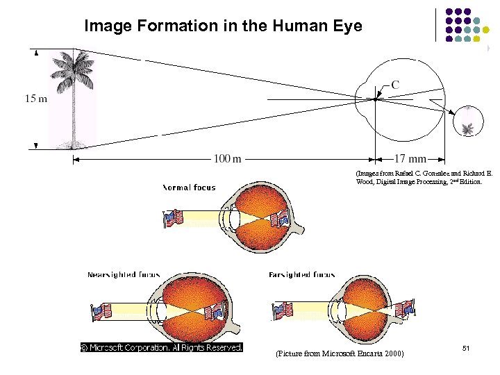 Image Formation in the Human Eye (Images from Rafael C. Gonzalez and Richard E. Wood, Digital Image Processing, 2 nd Edition. (Picture from Microsoft Encarta 2000) 51
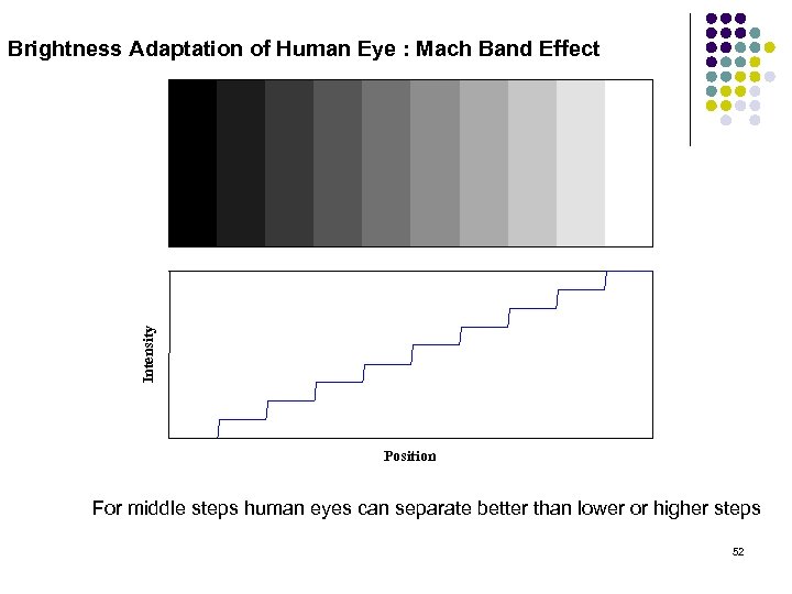 Intensity Brightness Adaptation of Human Eye : Mach Band Effect Position For middle steps human eyes can separate better than lower or higher steps 52
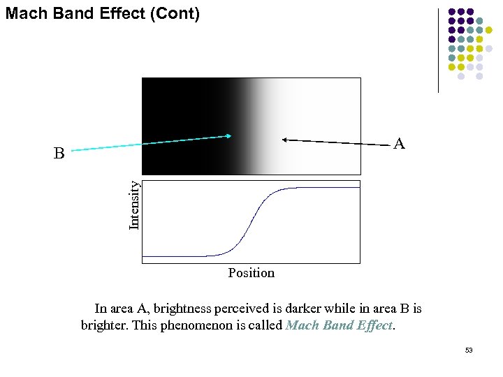 Mach Band Effect (Cont) A Intensity B Position In area A, brightness perceived is darker while in area B is brighter. This phenomenon is called Mach Band Effect. 53
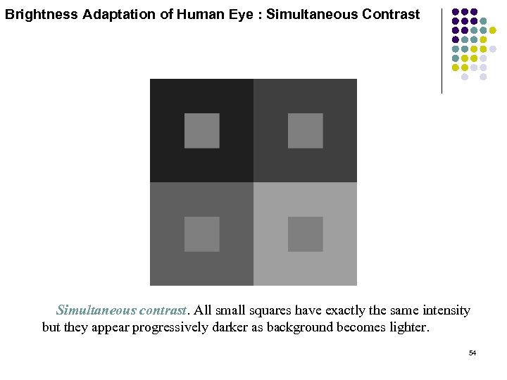 Brightness Adaptation of Human Eye : Simultaneous Contrast Simultaneous contrast. All small squares have exactly the same intensity but they appear progressively darker as background becomes lighter. 54
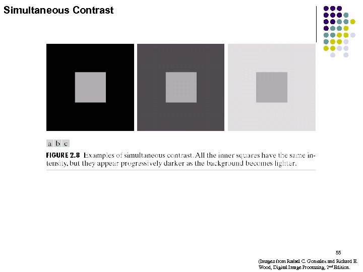 Simultaneous Contrast 55 (Images from Rafael C. Gonzalez and Richard E. Wood, Digital Image Processing, 2 nd Edition.
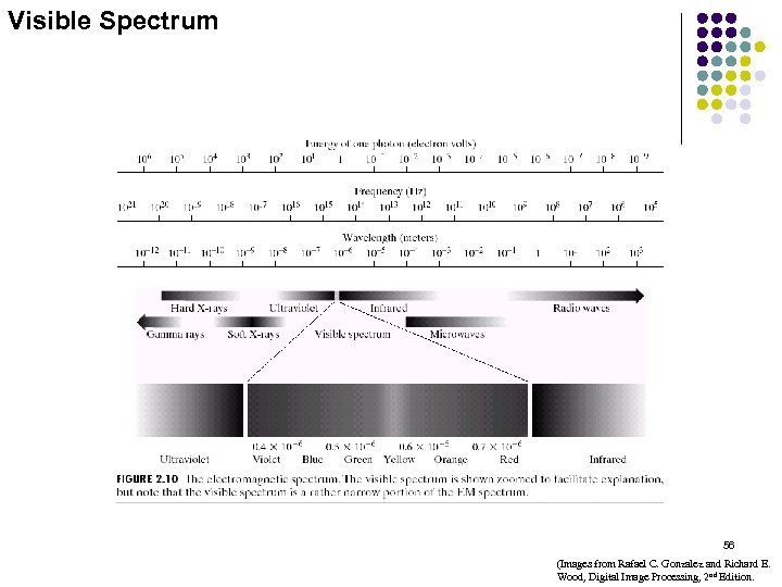 Visible Spectrum 56 (Images from Rafael C. Gonzalez and Richard E. Wood, Digital Image Processing, 2 nd Edition.
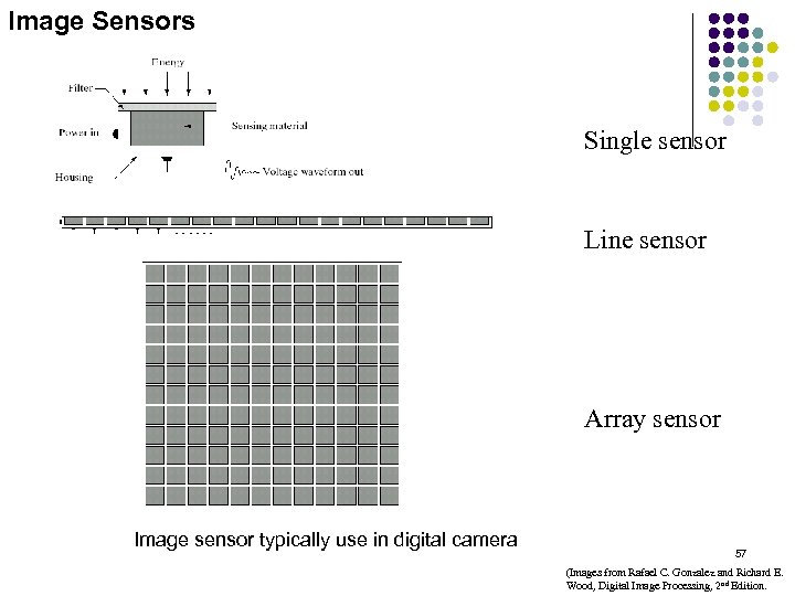 Image Sensors Single sensor Line sensor Array sensor Image sensor typically use in digital camera 57 (Images from Rafael C. Gonzalez and Richard E. Wood, Digital Image Processing, 2 nd Edition.
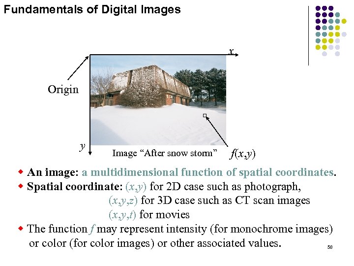 Fundamentals of Digital Images x Origin y Image “After snow storm” f(x, y) w An image: a multidimensional function of spatial coordinates. w Spatial coordinate: (x, y) for 2 D case such as photograph, (x, y, z) for 3 D case such as CT scan images (x, y, t) for movies w The function f may represent intensity (for monochrome images) or color (for color images) or other associated values. 58
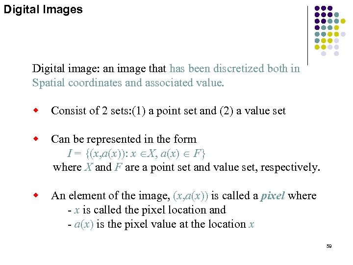 Digital Images Digital image: an image that has been discretized both in Spatial coordinates and associated value. w Consist of 2 sets: (1) a point set and (2) a value set w Can be represented in the form I = {(x, a(x)): x ÎX, a(x) Î F} where X and F are a point set and value set, respectively. w An element of the image, (x, a(x)) is called a pixel where - x is called the pixel location and - a(x) is the pixel value at the location x 59
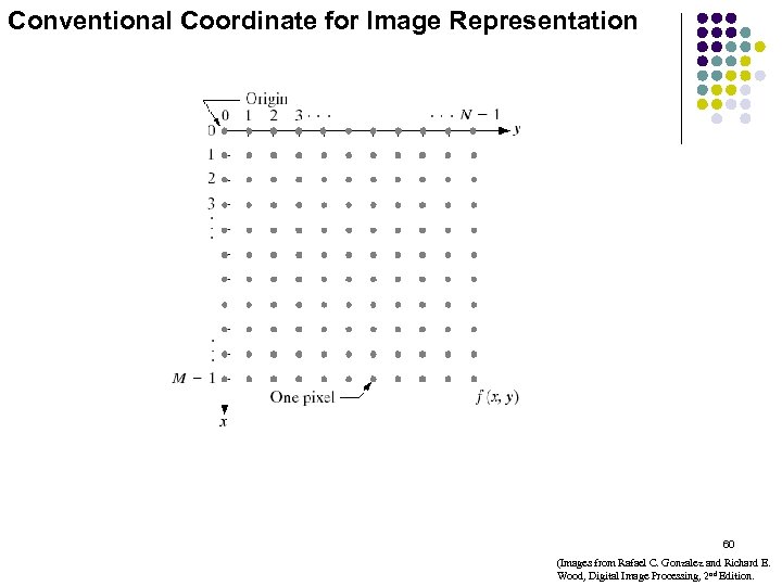 Conventional Coordinate for Image Representation 60 (Images from Rafael C. Gonzalez and Richard E. Wood, Digital Image Processing, 2 nd Edition.
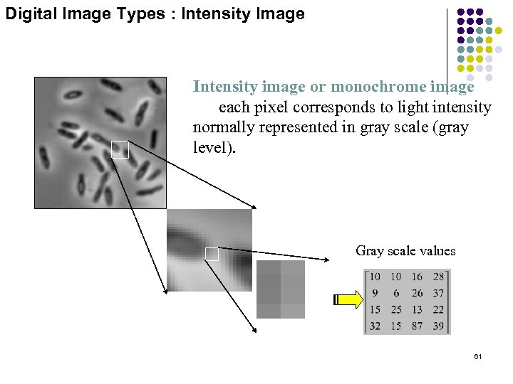 Digital Image Types : Intensity Image Intensity image or monochrome image each pixel corresponds to light intensity normally represented in gray scale (gray level). Gray scale values 61
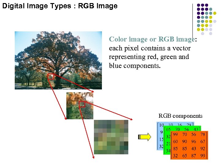 Digital Image Types : RGB Image Color image or RGB image: each pixel contains a vector representing red, green and blue components. RGB components 62
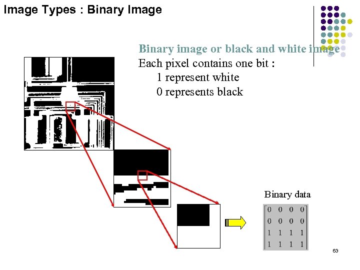 Image Types : Binary Image Binary image or black and white image Each pixel contains one bit : 1 represent white 0 represents black Binary data 63
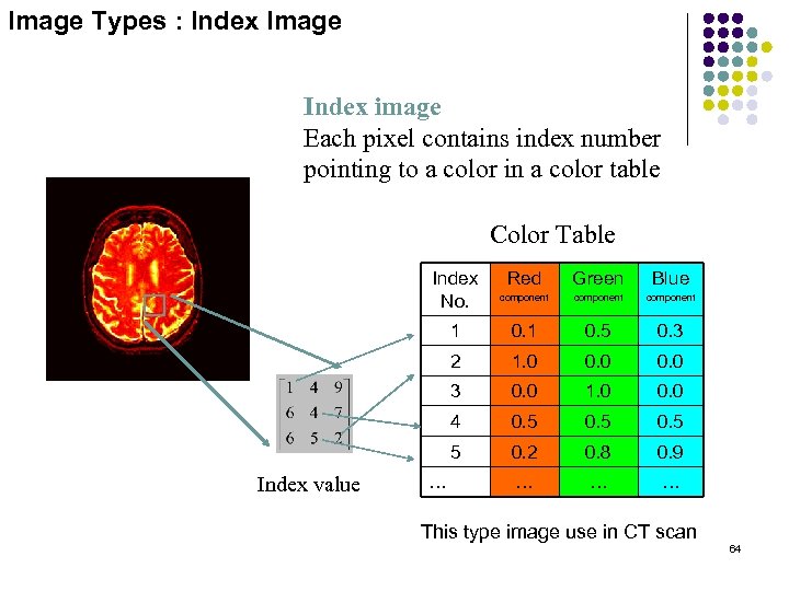 Image Types : Index Image Index image Each pixel contains index number pointing to a color in a color table Color Table Index No. Blue component 0. 1 0. 5 0. 3 2 1. 0 0. 0 3 0. 0 1. 0 0. 0 4 0. 5 5 … Green 1 Index value Red component 0. 2 0. 8 0. 9 … … … This type image use in CT scan 64
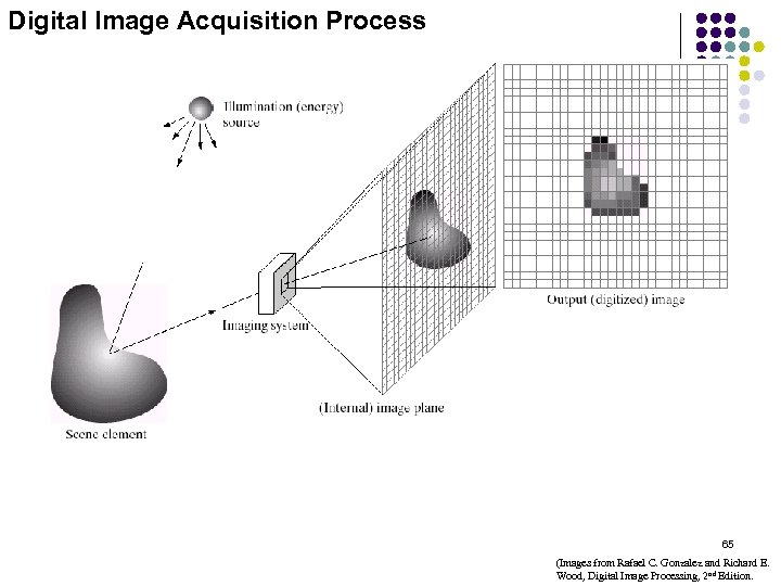 Digital Image Acquisition Process 65 (Images from Rafael C. Gonzalez and Richard E. Wood, Digital Image Processing, 2 nd Edition.
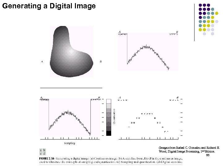 Generating a Digital Image (Images from Rafael C. Gonzalez and Richard E. Wood, Digital Image Processing, 2 nd Edition. 66
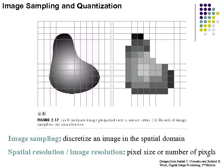 Image Sampling and Quantization Image sampling: discretize an image in the spatial domain Spatial resolution / image resolution: pixel size or number of pixels 67 (Images from Rafael C. Gonzalez and Richard E. Wood, Digital Image Processing, 2 nd Edition.
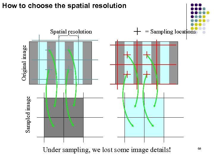 How to choose the spatial resolution = Sampling locations Sampled image Original image Spatial resolution Under sampling, we lost some image details! 68
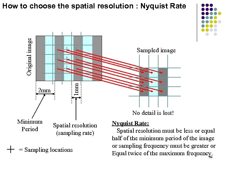 Original image How to choose the spatial resolution : Nyquist Rate 2 mm 1 mm Sampled image No detail is lost! Minimum Period Spatial resolution (sampling rate) = Sampling locations Nyquist Rate: Spatial resolution must be less or equal half of the minimum period of the image or sampling frequency must be greater or Equal twice of the maximum frequency. 69
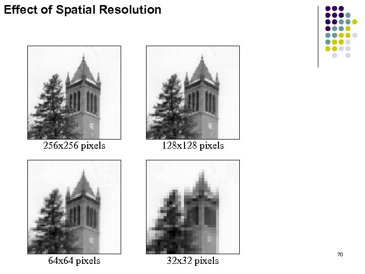 Effect of Spatial Resolution 256 x 256 pixels 128 x 128 pixels 64 x 64 pixels 32 x 32 pixels 70
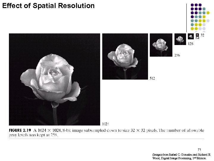 Effect of Spatial Resolution 71 (Images from Rafael C. Gonzalez and Richard E. Wood, Digital Image Processing, 2 nd Edition.
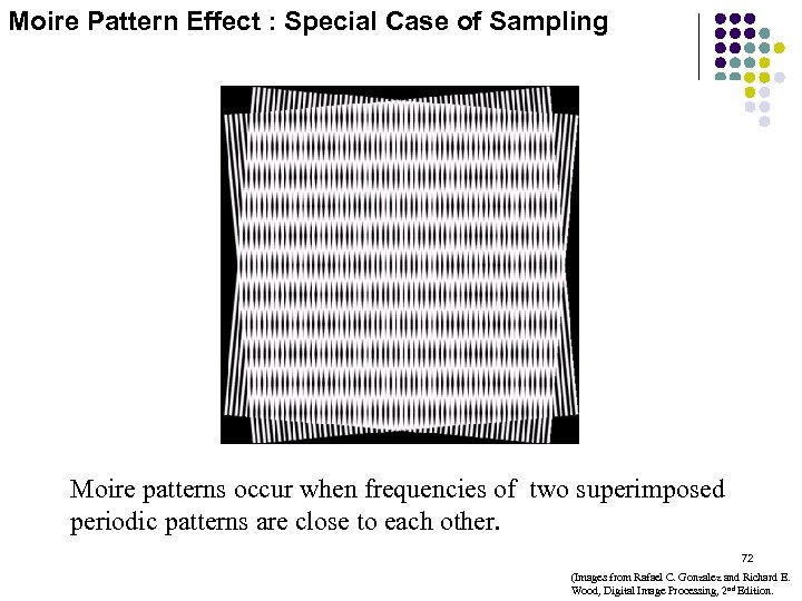 Moire Pattern Effect : Special Case of Sampling Moire patterns occur when frequencies of two superimposed periodic patterns are close to each other. 72 (Images from Rafael C. Gonzalez and Richard E. Wood, Digital Image Processing, 2 nd Edition.
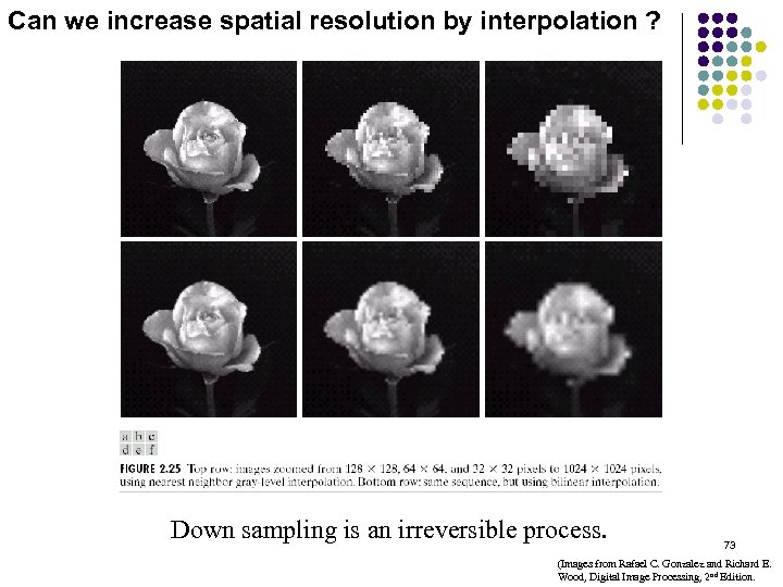 Can we increase spatial resolution by interpolation ? Down sampling is an irreversible process. 73 (Images from Rafael C. Gonzalez and Richard E. Wood, Digital Image Processing, 2 nd Edition.
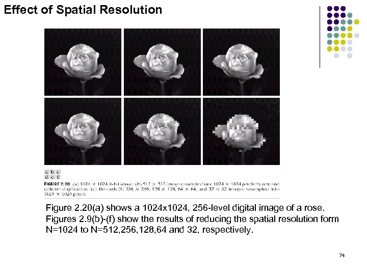 Effect of Spatial Resolution Figure 2. 20(a) shows a 1024 x 1024, 256 -level digital image of a rose. Figures 2. 9(b)-(f) show the results of reducing the spatial resolution form N=1024 to N=512, 256, 128, 64 and 32, respectively. 74
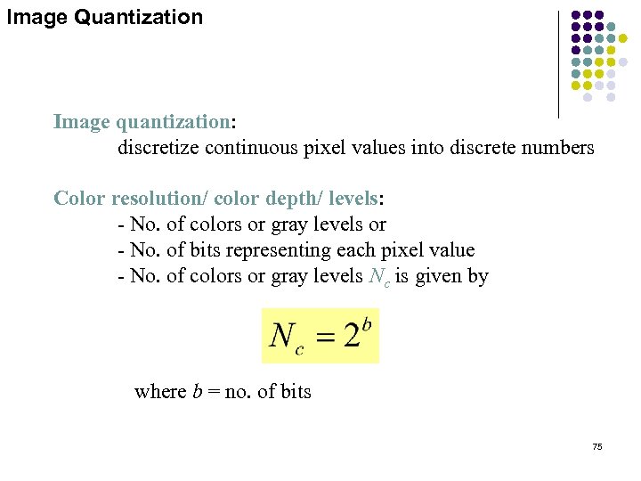 Image Quantization Image quantization: discretize continuous pixel values into discrete numbers Color resolution/ color depth/ levels: - No. of colors or gray levels or - No. of bits representing each pixel value - No. of colors or gray levels Nc is given by where b = no. of bits 75
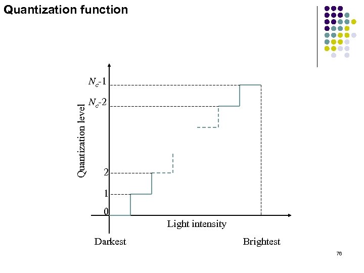 Quantization function Quantization level Nc-1 Nc-2 2 1 0 Light intensity Darkest Brightest 76
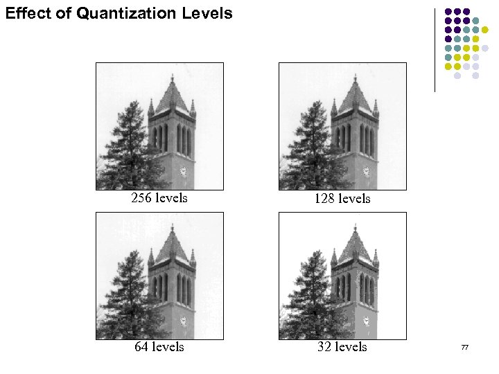 Effect of Quantization Levels 256 levels 128 levels 64 levels 32 levels 77
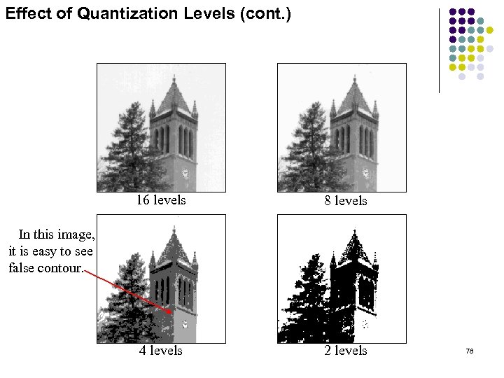 Effect of Quantization Levels (cont. ) 16 levels 8 levels 4 levels 2 levels In this image, it is easy to see false contour. 78
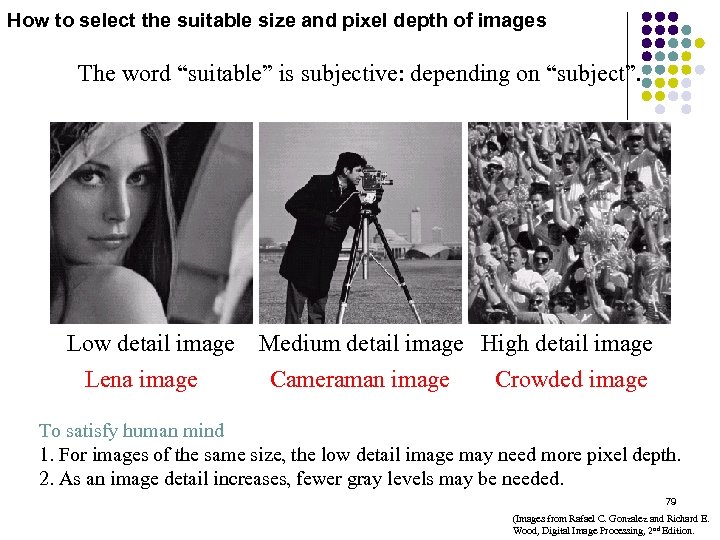 How to select the suitable size and pixel depth of images The word “suitable” is subjective: depending on “subject”. Low detail image Lena image Medium detail image High detail image Cameraman image Crowded image To satisfy human mind 1. For images of the same size, the low detail image may need more pixel depth. 2. As an image detail increases, fewer gray levels may be needed. 79 (Images from Rafael C. Gonzalez and Richard E. Wood, Digital Image Processing, 2 nd Edition.
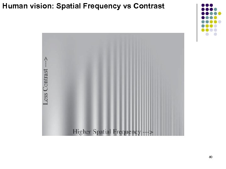 Human vision: Spatial Frequency vs Contrast 80
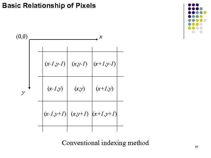 Basic Relationship of Pixels (0, 0) x (x-1, y-1) y (x, y-1) (x+1, y-1) (x-1, y) (x+1, y) (x-1, y+1) (x+1, y+1) Conventional indexing method 81
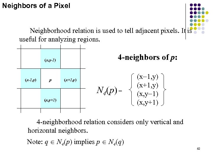 Neighbors of a Pixel Neighborhood relation is used to tell adjacent pixels. It is useful for analyzing regions. 4 -neighbors of p: (x, y-1) (x-1, y) p (x+1, y) N 4(p) = (x, y+1) (x-1, y) (x+1, y) (x, y-1) (x, y+1) 4 -neighborhood relation considers only vertical and horizontal neighbors. Note: q Î N 4(p) implies p Î N 4(q) 82
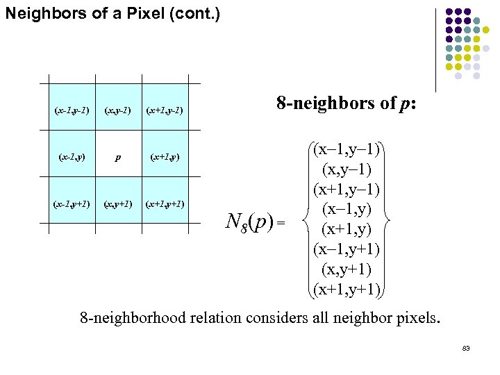 Neighbors of a Pixel (cont. ) (x-1, y-1) (x+1, y-1) (x-1, y) p (x+1, y) (x-1, y+1) (x+1, y+1) 8 -neighbors of p: N 8(p) = (x-1, y-1) (x+1, y-1) (x-1, y) (x+1, y) (x-1, y+1) (x+1, y+1) 8 -neighborhood relation considers all neighbor pixels. 83
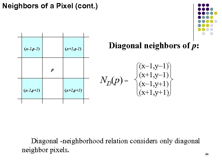 Neighbors of a Pixel (cont. ) (x-1, y-1) (x+1, y-1) Diagonal neighbors of p: p ND(p) = (x-1, y+1) (x+1, y+1) (x-1, y-1) (x+1, y-1) (x-1, y+1) (x+1, y+1) Diagonal -neighborhood relation considers only diagonal neighbor pixels. 84
 Connectivity is adapted from neighborhood relation. Two pixels are connected if they are in the same class (i. e. the same color or the same range of intensity) and they are neighbors of one another. For p and q from the same class w 4 -connectivity: p and q are 4 -connected if q Î N 4(p) w 8 -connectivity: p and q are 8 -connected if q Î N 8(p) w mixed-connectivity (m-connectivity): p and q are m-connected if q Î N 4(p) or q Î ND(p) and N 4(p) Ç N 4(q) = Æ 85
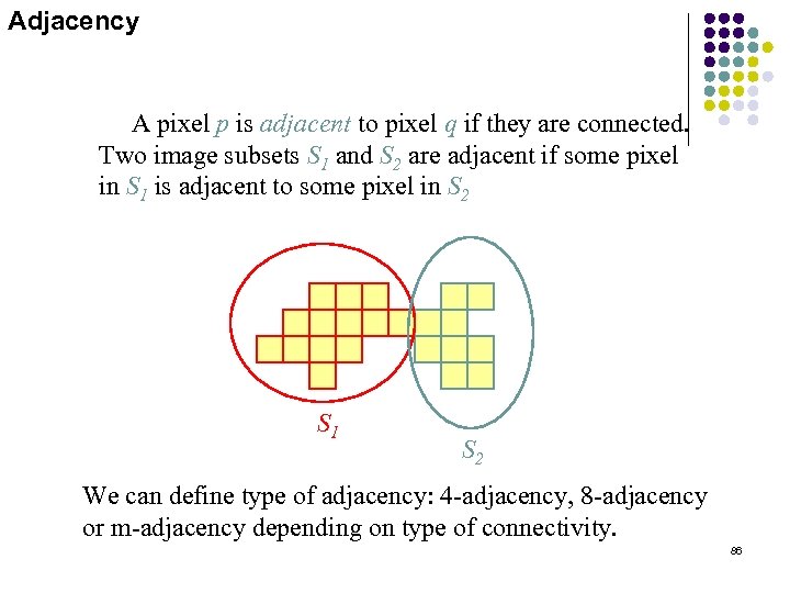 Adjacency A pixel p is adjacent to pixel q if they are connected. Two image subsets S 1 and S 2 are adjacent if some pixel in S 1 is adjacent to some pixel in S 2 S 1 S 2 We can define type of adjacency: 4 -adjacency, 8 -adjacency or m-adjacency depending on type of connectivity. 86
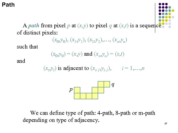 Path A path from pixel p at (x, y) to pixel q at (s, t) is a sequence of distinct pixels: (x 0, y 0), (x 1, y 1), (x 2, y 2), …, (xn, yn) such that (x 0, y 0) = (x, y) and (xn, yn) = (s, t) and (xi, yi) is adjacent to (xi-1, yi-1), i = 1, …, n p q We can define type of path: 4 -path, 8 -path or m-path depending on type of adjacency. 87
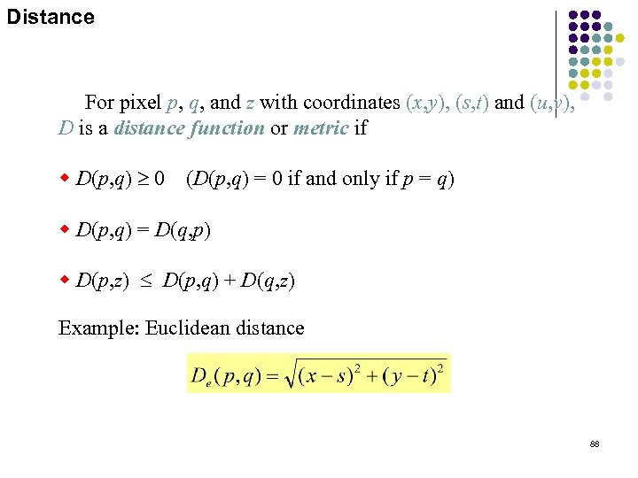 Distance For pixel p, q, and z with coordinates (x, y), (s, t) and (u, v), D is a distance function or metric if w D(p, q) ³ 0 (D(p, q) = 0 if and only if p = q) w D(p, q) = D(q, p) w D(p, z) £ D(p, q) + D(q, z) Example: Euclidean distance 88
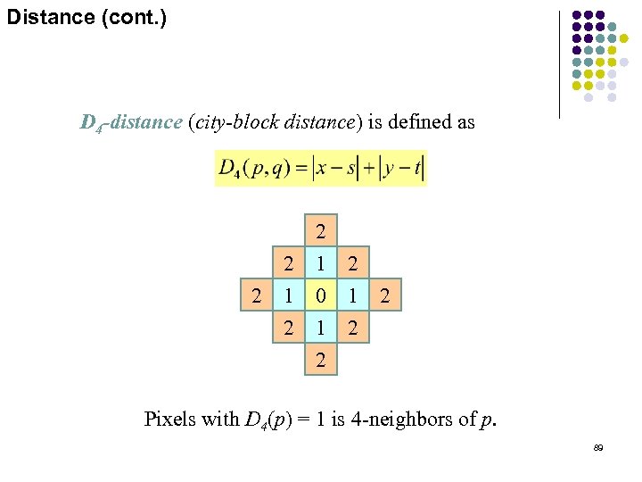 Distance (cont. ) D 4 -distance (city-block distance) is defined as 2 2 2 1 0 1 2 2 Pixels with D 4(p) = 1 is 4 -neighbors of p. 89
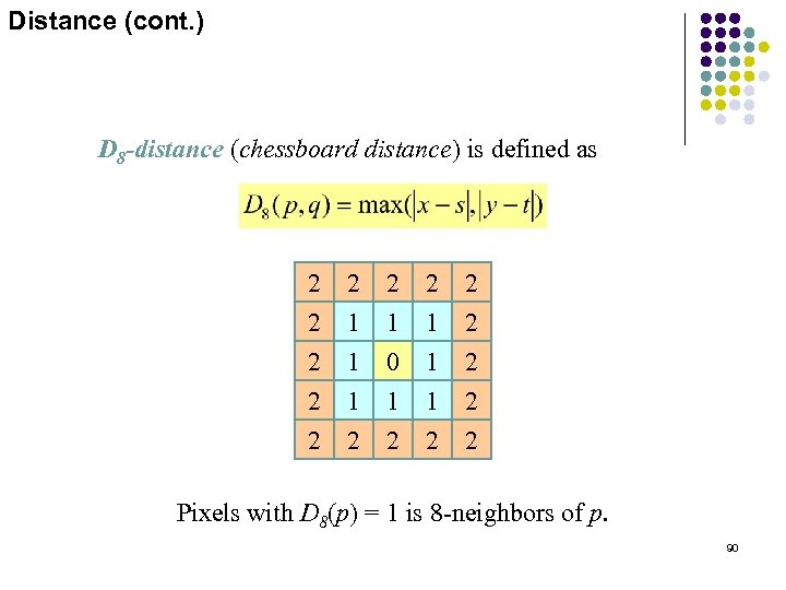 Distance (cont. ) D 8 -distance (chessboard distance) is defined as 2 2 2 2 2 1 1 1 2 1 0 1 2 1 1 1 2 2 2 Pixels with D 8(p) = 1 is 8 -neighbors of p. 90
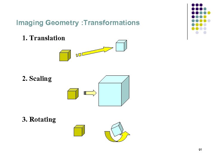 Imaging Geometry : Transformations 1. Translation 2. Scaling 3. Rotating 91
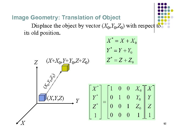 Image Geometry: Translation of Object Displace the object by vector (X 0, Y 0, Z 0) with respect to its old position. (X+X 0, Y+Y 0, Z+Z 0) (X 0 , Y 0 , Z 0) Z (X, Y, Z) X Y 92
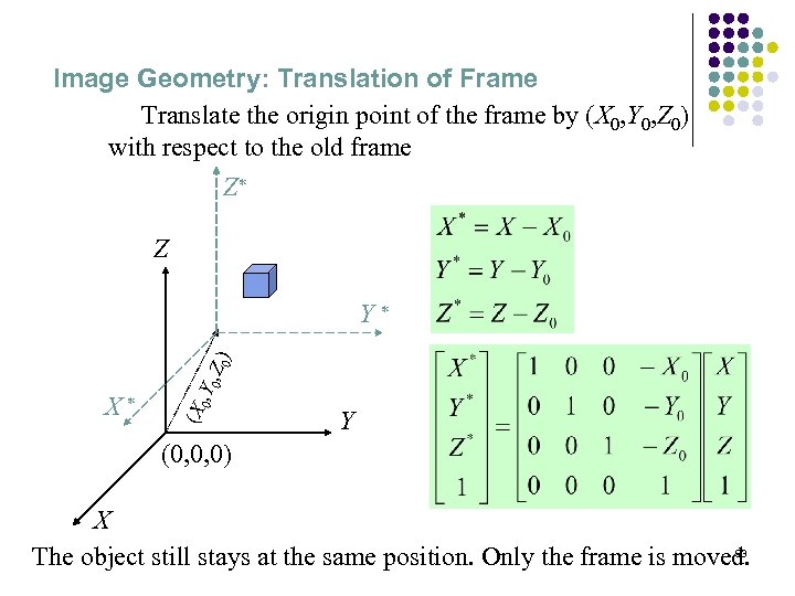 Image Geometry: Translation of Frame Translate the origin point of the frame by (X 0, Y 0, Z 0) with respect to the old frame Z* Z (X X* 0 , Y 0 , Z 0) Y* Y (0, 0, 0) X 93 The object still stays at the same position. Only the frame is moved.
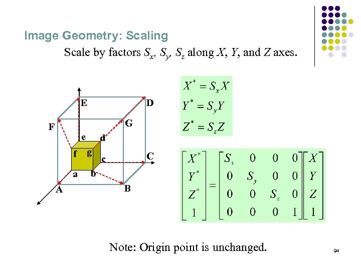 Image Geometry: Scaling Scale by factors Sx, Sy, Sz along X, Y, and Z axes. E D G F e f a A d g C c b B Note: Origin point is unchanged. 94
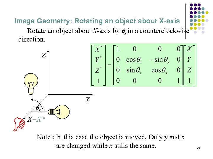 Image Geometry: Rotating an object about X-axis Rotate an object about X-axis by qx in a counterclockwise direction. Z qx Y X=X * D Note : In this case the object is moved. Only y and z are changed while x stills the same. 95
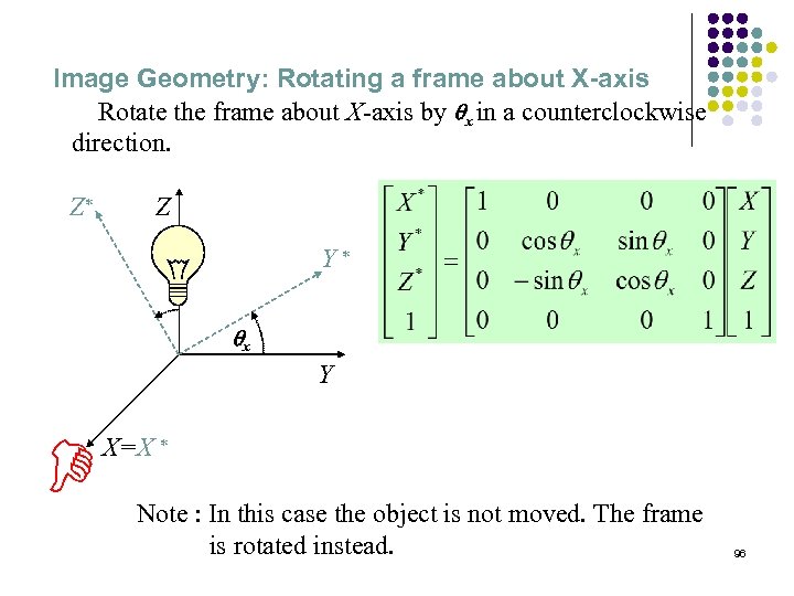 Image Geometry: Rotating a frame about X-axis Rotate the frame about X-axis by qx in a counterclockwise direction. Z* Z Y* qx Y X=X * D Note : In this case the object is not moved. The frame is rotated instead. 96
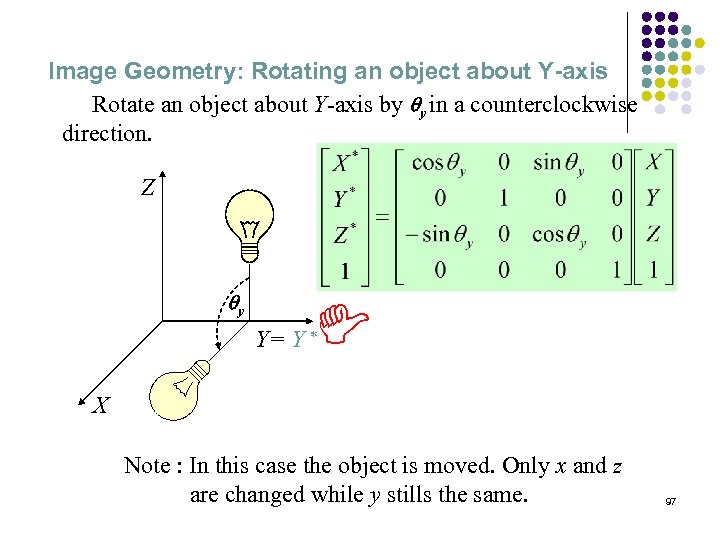 Image Geometry: Rotating an object about Y-axis Rotate an object about Y-axis by qy in a counterclockwise direction. qy D Z Y= Y * X Note : In this case the object is moved. Only x and z are changed while y stills the same. 97
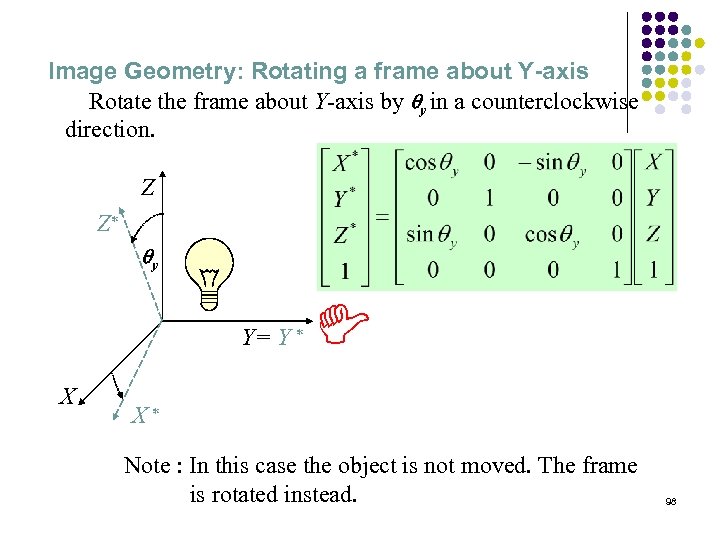 Image Geometry: Rotating a frame about Y-axis Rotate the frame about Y-axis by qy in a counterclockwise direction. Z Z* D qy Y= Y * X X* Note : In this case the object is not moved. The frame is rotated instead. 98
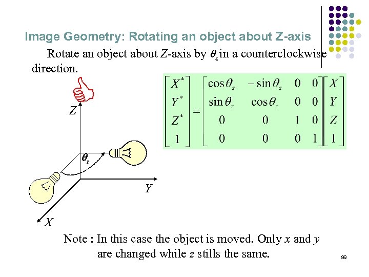 Image Geometry: Rotating an object about Z-axis Rotate an object about Z-axis by qz in a counterclockwise direction. D Z qz Y X Note : In this case the object is moved. Only x and y are changed while z stills the same. 99
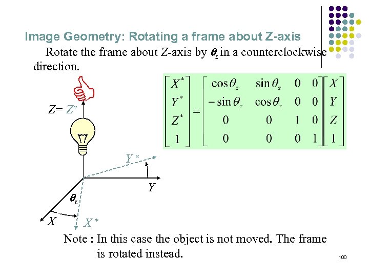 Image Geometry: Rotating a frame about Z-axis Rotate the frame about Z-axis by qz in a counterclockwise direction. D Z= Z* Y* qz X Y X* Note : In this case the object is not moved. The frame is rotated instead. 100
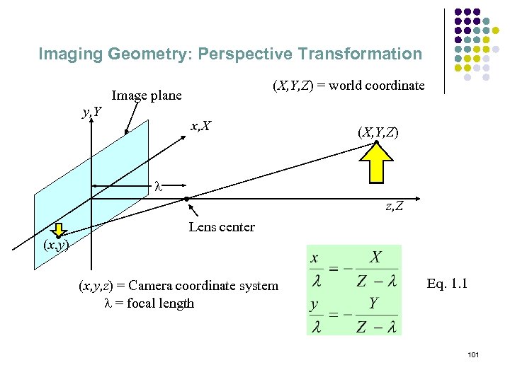 Imaging Geometry: Perspective Transformation (X, Y, Z) = world coordinate Image plane y, Y x, X (X, Y, Z) l z, Z Lens center (x, y) (x, y, z) = Camera coordinate system l = focal length Eq. 1. 1 101
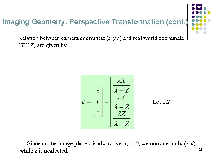 Imaging Geometry: Perspective Transformation (cont. ) Relation between camera coordinate (x, y, z) and real world coordinate (X, Y, Z) are given by Eq. 1. 2 Since on the image plane z is always zero, z=0, we consider only (x, y) 102 while z is neglected.
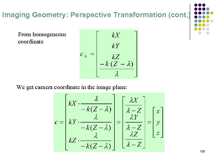
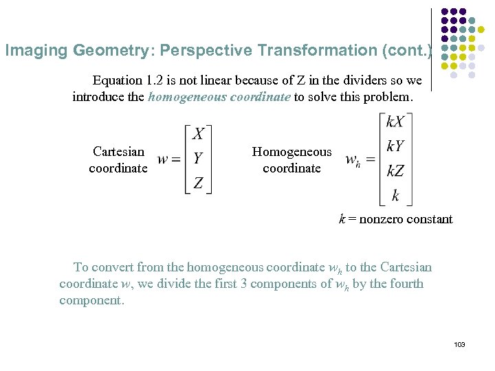 Imaging Geometry: Perspective Transformation (cont. ) Equation 1. 2 is not linear because of Z in the dividers so we introduce the homogeneous coordinate to solve this problem. Cartesian coordinate Homogeneous coordinate k = nonzero constant To convert from the homogeneous coordinate wh to the Cartesian coordinate w, we divide the first 3 components of wh by the fourth component. 103
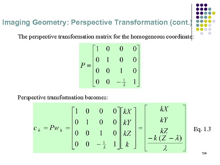 Imaging Geometry: Perspective Transformation (cont. ) The perspective transformation matrix for the homogeneous coordinate: Perspective transformation becomes: Eq. 1. 3 104
 Imaging Geometry: Perspective Transformation (cont. ) From homogeneous coordinate We get camera coordinate in the image plane: 105
 Imaging Geometry: Inverse Perspective Transformation where Eq. 1. 4 106
 Inverse Perspective Transformation (cont. ) For an image point (x 0, y 0), since on the image plane z=0, we have We get the real world coordinate : Since the perspective transformation maps 3 -D coordinates to 2 -D Coordinates, we cannot get the inverse transform. 107
 Inverse Perspective Transformation (cont. ) To find the solution, let We get Eq. 1. 5 108
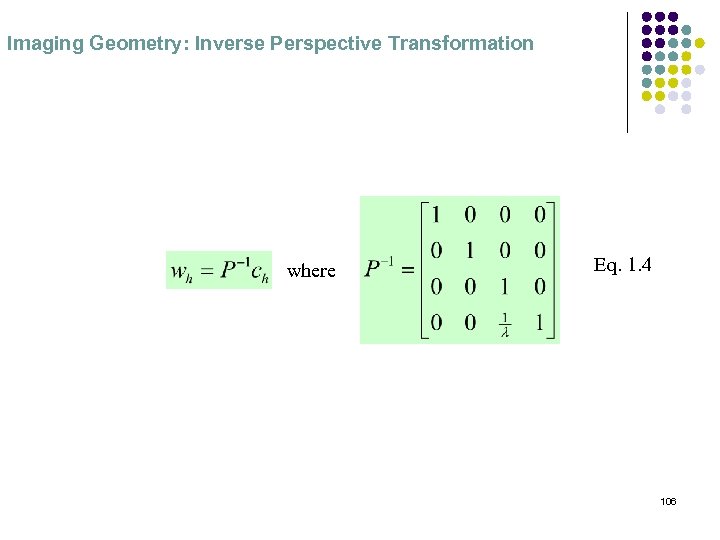
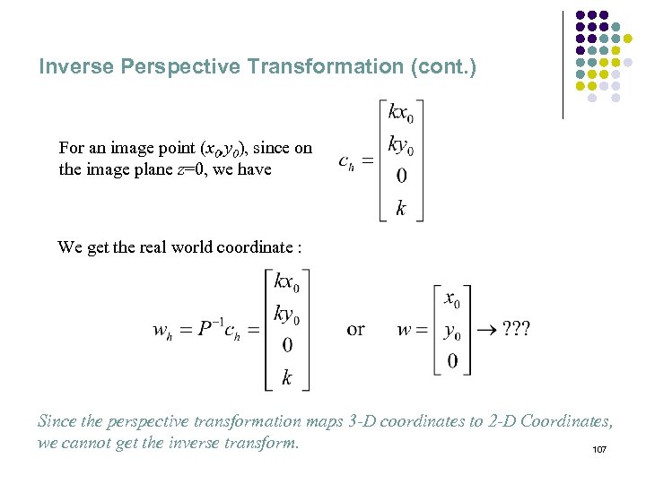
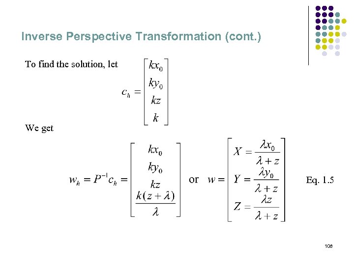
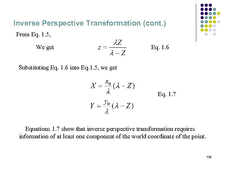 Inverse Perspective Transformation (cont. ) From Eq. 1. 5, We get Eq. 1. 6 Substituting Eq. 1. 6 into Eq. 1. 5, we get Eq. 1. 7 Equations 1. 7 show that inverse perspective transformation requires information of at least one component of the world coordinate of the point. 109
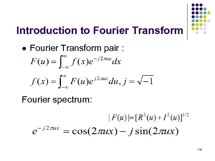 Introduction to Fourier Transform l Fourier Transform pair : Fourier spectrum: 110
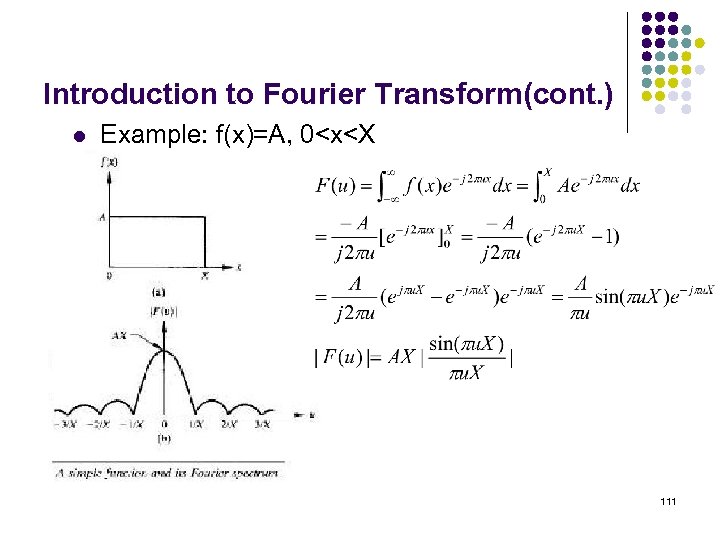 Introduction to Fourier Transform(cont. ) l Example: f(x)=A, 0
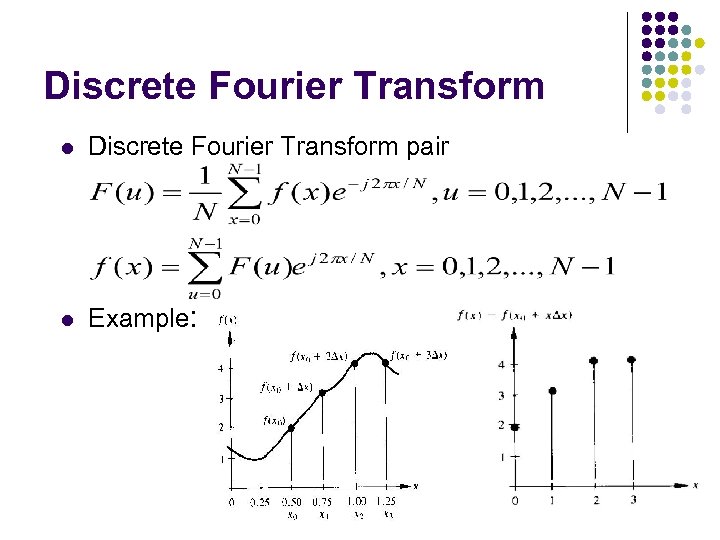 Discrete Fourier Transform l Discrete Fourier Transform pair l Example: 112
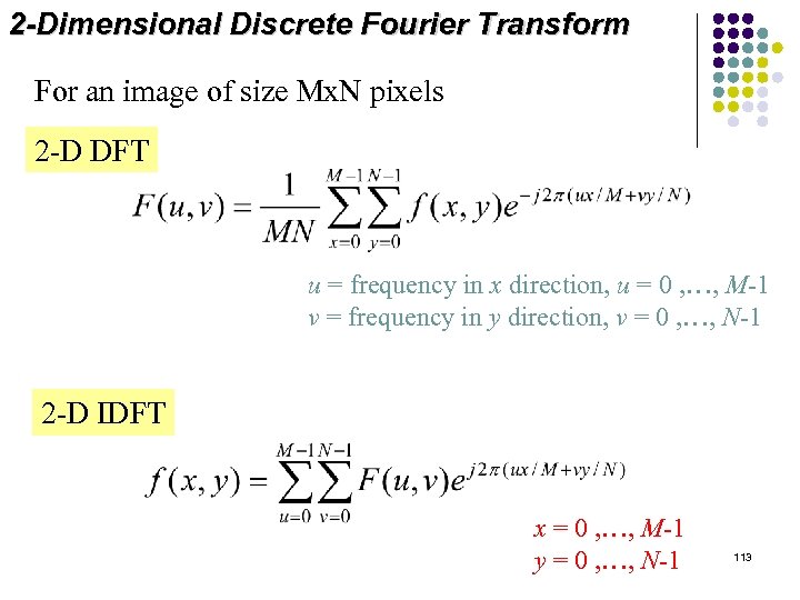 2 -Dimensional Discrete Fourier Transform For an image of size Mx. N pixels 2 -D DFT u = frequency in x direction, u = 0 , …, M-1 v = frequency in y direction, v = 0 , …, N-1 2 -D IDFT x = 0 , …, M-1 y = 0 , …, N-1 113
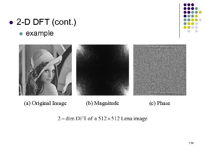 l 2 -D DFT (cont. ) l example (a) Original Image (b) Magnitude (c) Phase 114
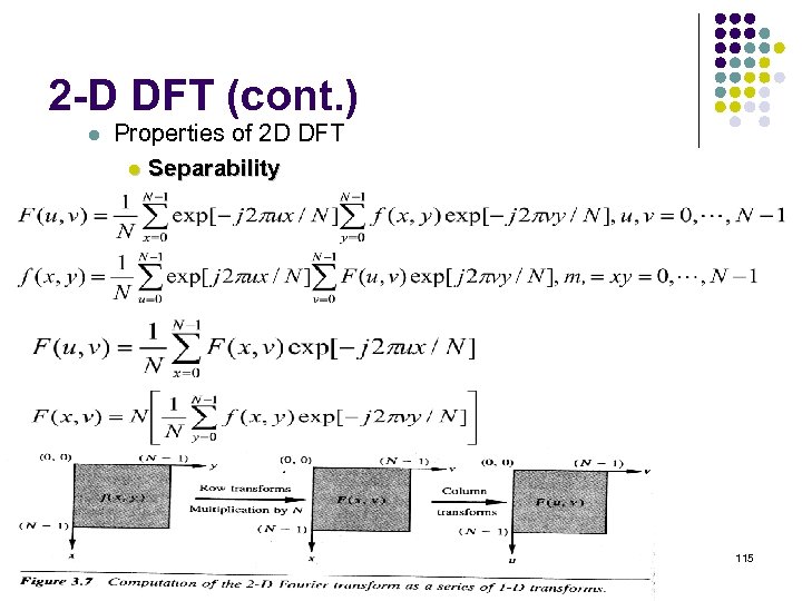 2 -D DFT (cont. ) l Properties of 2 D DFT l Separability 115
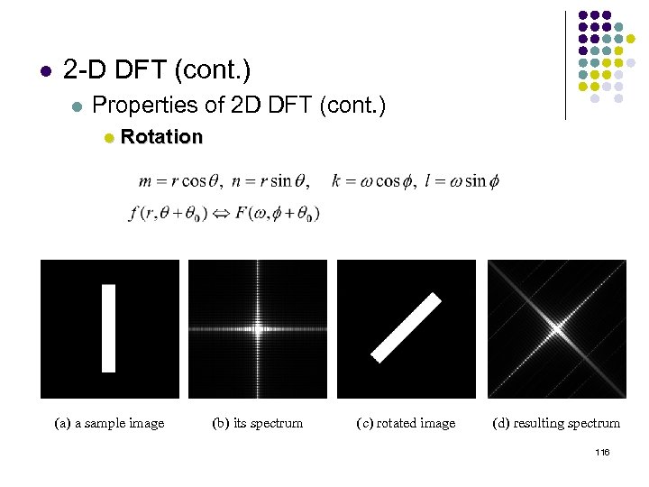 l 2 -D DFT (cont. ) l Properties of 2 D DFT (cont. ) l Rotation (a) a sample image (b) its spectrum (c) rotated image (d) resulting spectrum 116
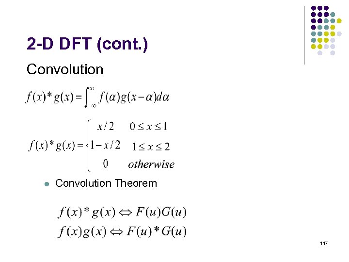 2 -D DFT (cont. ) Convolution l Convolution Theorem 117
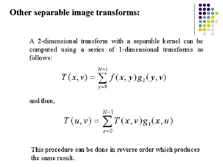 Other separable image transforms: 118
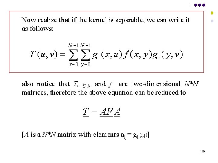 119
119
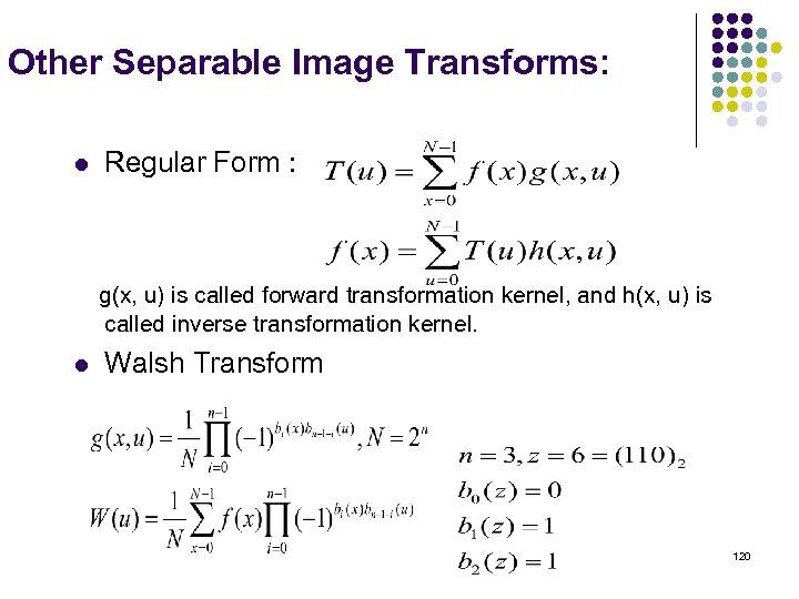 Other Separable Image Transforms: l Regular Form : g(x, u) is called forward transformation kernel, and h(x, u) is called inverse transformation kernel. l Walsh Transform 120
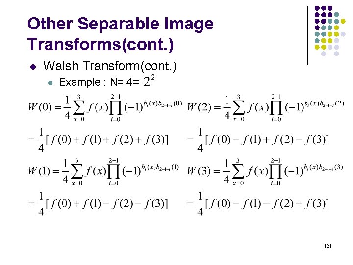 Other Separable Image Transforms(cont. ) l Walsh Transform(cont. ) l Example : N= 4= 121
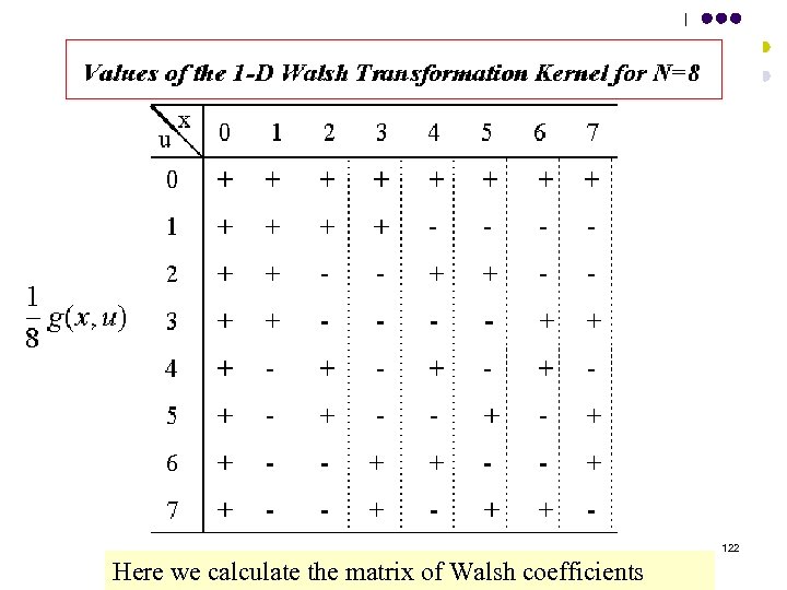 122 Here we calculate the matrix of Walsh coefficients
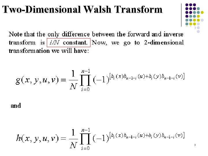 Two-Dimensional Walsh Transform 123
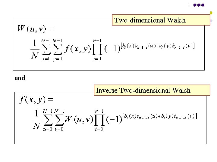 Two-dimensional Walsh Inverse Two-dimensional Walsh 124
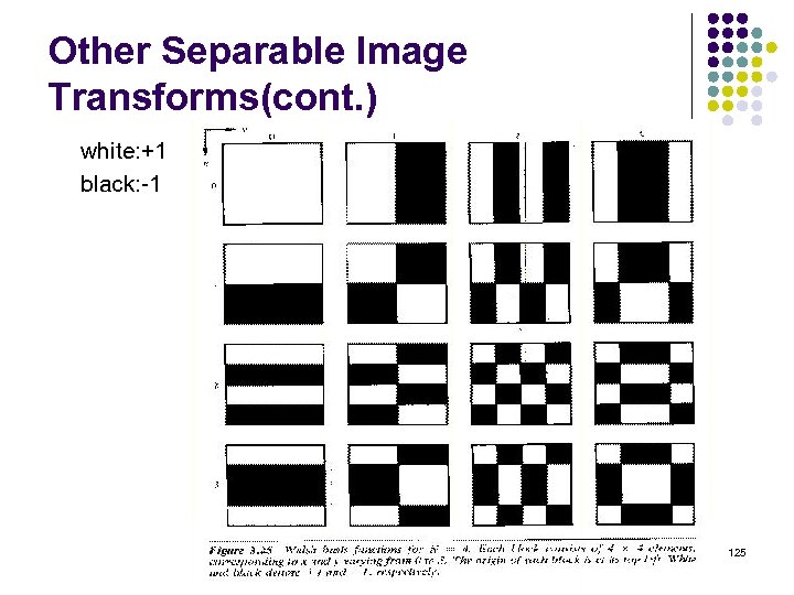 Other Separable Image Transforms(cont. ) white: +1 black: -1 125
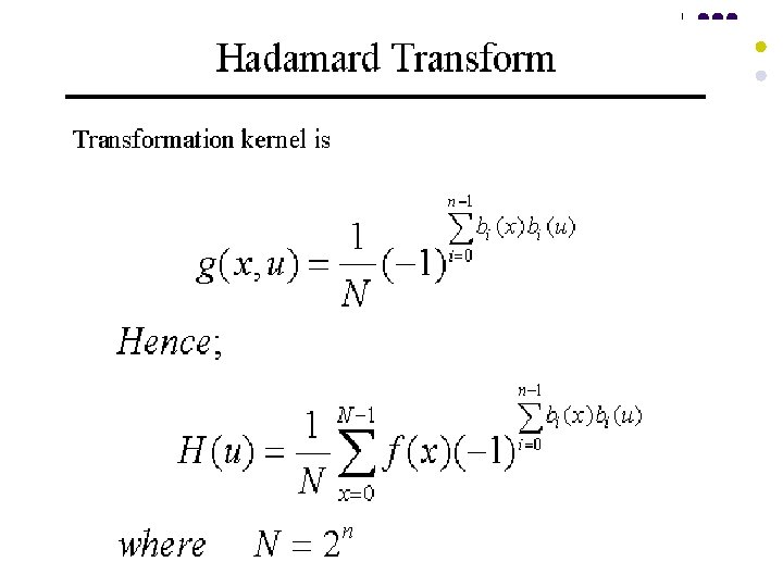 126
126
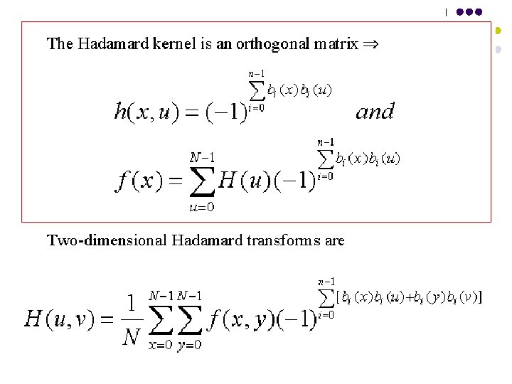 127
127
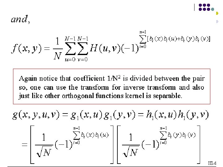 128
128
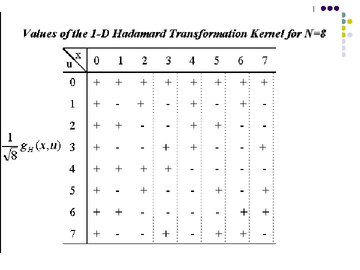 129
129
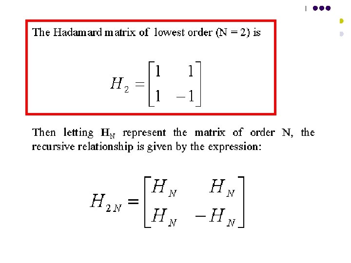 130
130
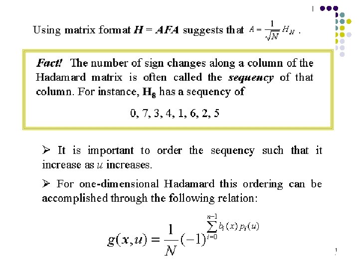 131
131
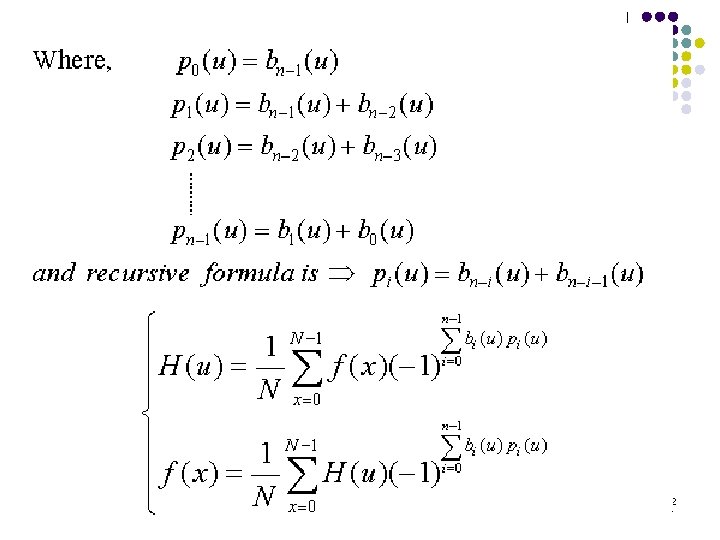 132
132
 133
133
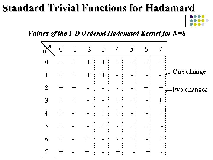 Standard Trivial Functions for Hadamard One change two changes 134
 135
135
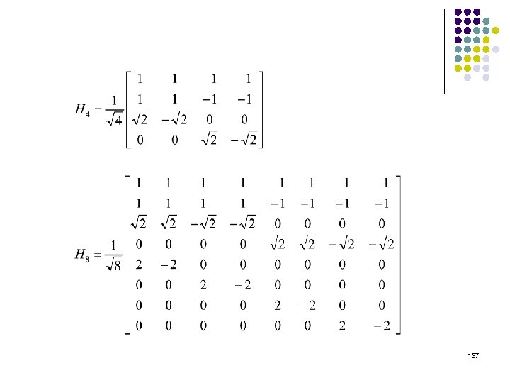
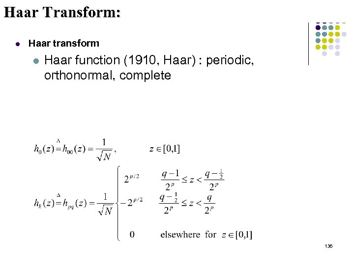 Haar Transform: l Haar transform l Haar function (1910, Haar) : periodic, orthonormal, complete 136
 137
137
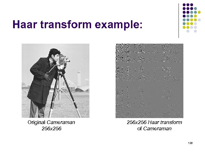 Haar transform example: Original Cameraman 256 x 256 Haar transform of Cameraman 138
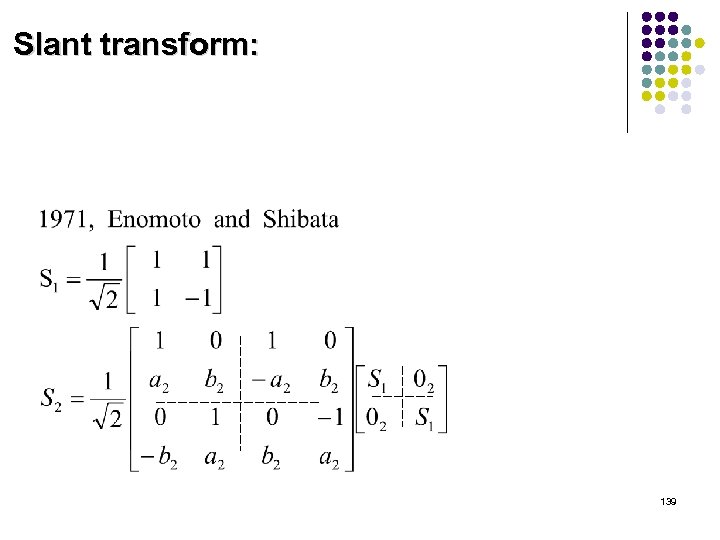 Slant transform: 139
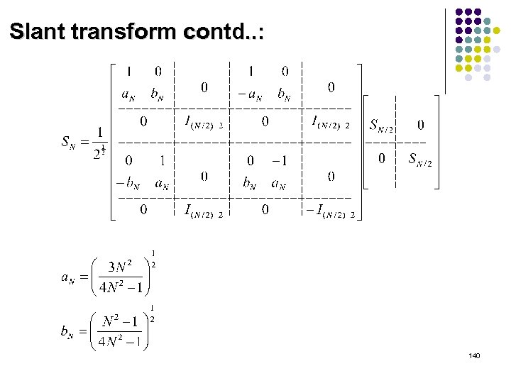 Slant transform contd. . : 140
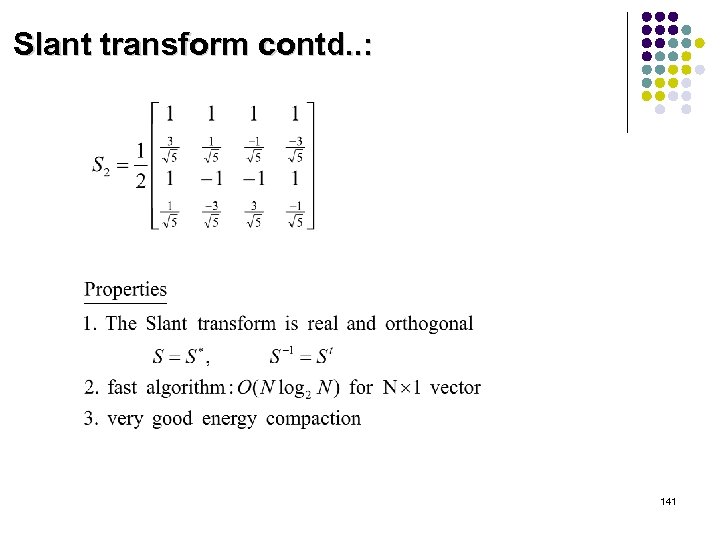 Slant transform contd. . : 141
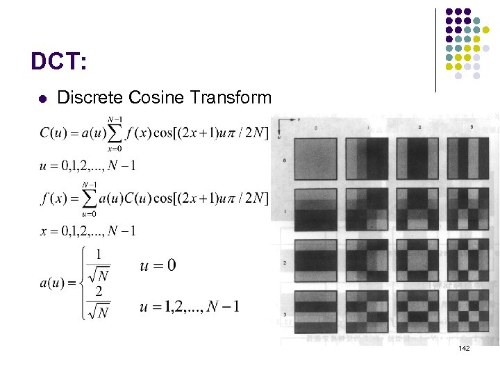 DCT: l Discrete Cosine Transform 142
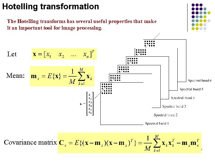 Hotelling transformation The Hotelling transforms has several useful properties that make it an important tool for image processing. Let Mean: Covariance matrix 143
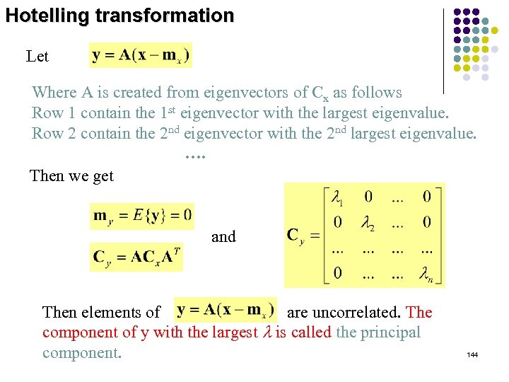 Hotelling transformation Let Where A is created from eigenvectors of Cx as follows Row 1 contain the 1 st eigenvector with the largest eigenvalue. Row 2 contain the 2 nd eigenvector with the 2 nd largest eigenvalue. …. Then we get and Then elements of are uncorrelated. The component of y with the largest l is called the principal component. 144
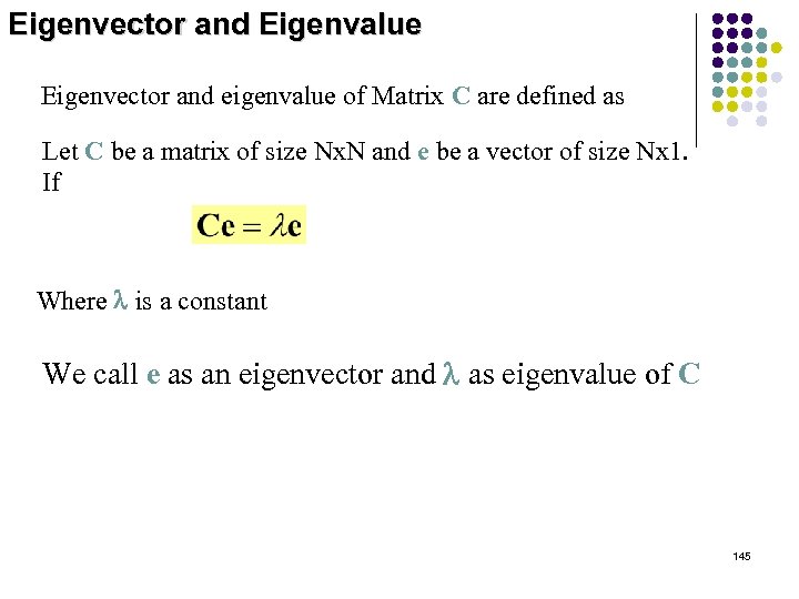 Eigenvector and Eigenvalue Eigenvector and eigenvalue of Matrix C are defined as Let C be a matrix of size Nx. N and e be a vector of size Nx 1. If Where l is a constant We call e as an eigenvector and l as eigenvalue of C 145
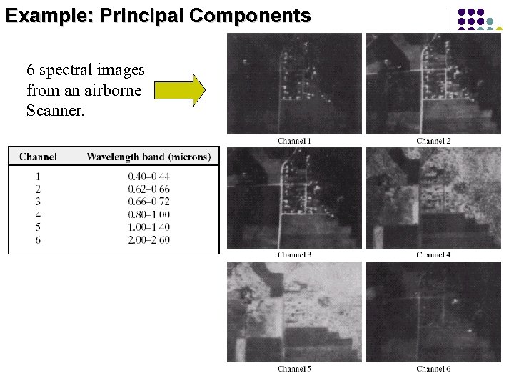 Example: Principal Components 6 spectral images from an airborne Scanner. 146
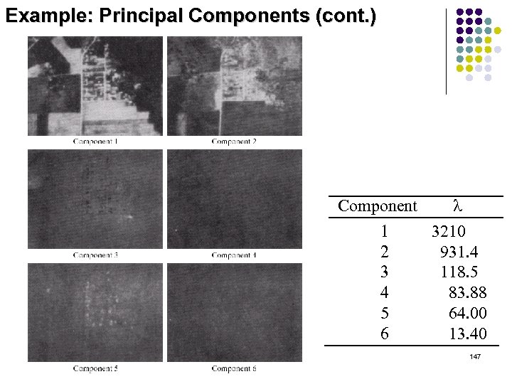 Example: Principal Components (cont. ) Component l 1 3210 2 931. 4 3 118. 5 4 83. 88 5 64. 00 6 13. 40 147
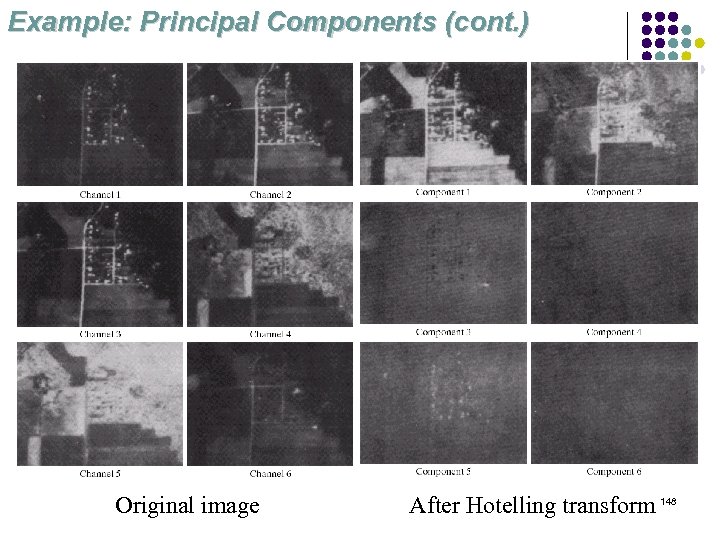 Example: Principal Components (cont. ) Original image After Hotelling transform 148
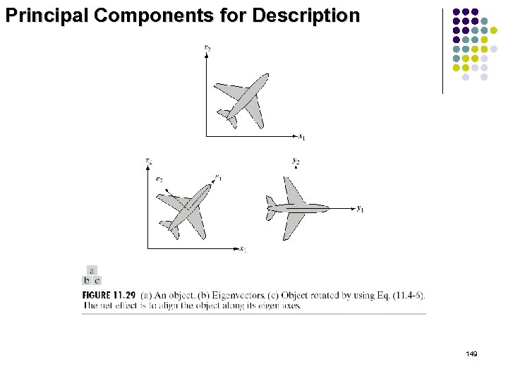 Principal Components for Description 149
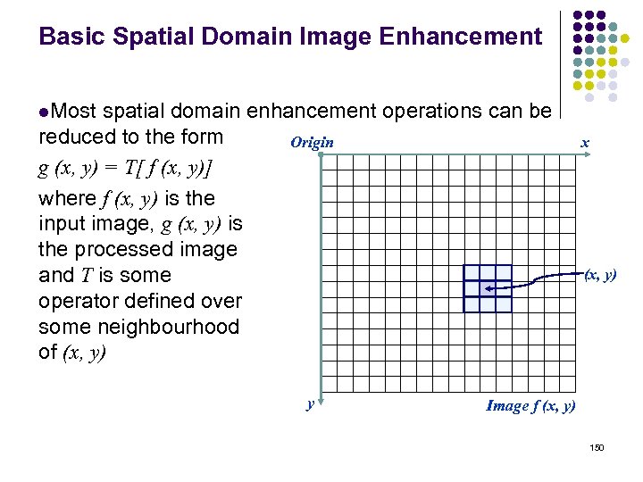 Basic Spatial Domain Image Enhancement l. Most spatial domain enhancement operations can be reduced to the form Origin g (x, y) = T[ f (x, y)] where f (x, y) is the input image, g (x, y) is the processed image and T is some operator defined over some neighbourhood of (x, y) y x (x, y) Image f (x, y) 150
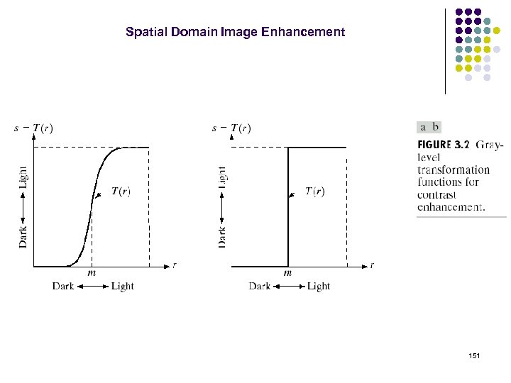 Spatial Domain Image Enhancement 151
 Point Processing l. The simplest spatial domain operations occur when the neighbourhood is simply the pixel itself In this case T is referred to as a grey level transformation function or a point processing operation Point processing operations take the form s=T(r) where s refers to the processed image pixel value and r refers to the original image pixel value 152
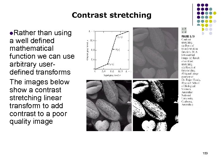 Contrast stretching l. Rather than using a well defined mathematical function we can use arbitrary userdefined transforms The images below show a contrast stretching linear transform to add contrast to a poor quality image 153
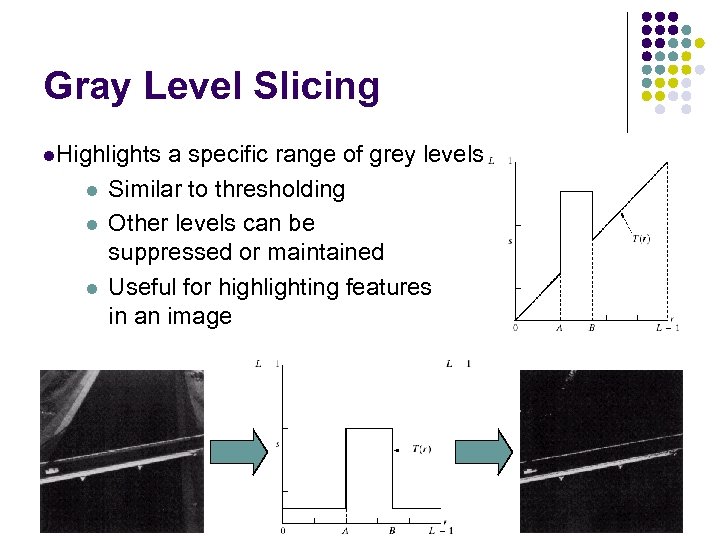 Gray Level Slicing l. Highlights l l l a specific range of grey levels Similar to thresholding Other levels can be suppressed or maintained Useful for highlighting features in an image 154
 Logarithmic Transformations l. The general form of the log transformation is s = c * log(1 + r) l. The log transformation maps a narrow range of low input grey level values into a wider range of output values l. The inverse log transformation performs the opposite transformation 155
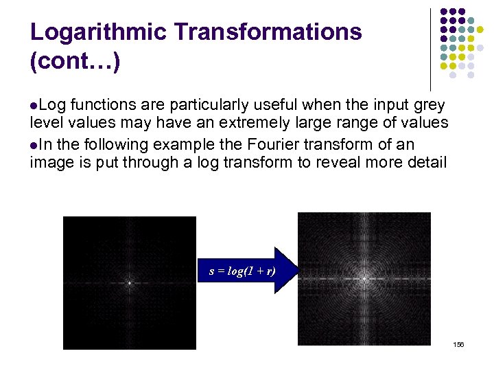 Logarithmic Transformations (cont…) l. Log functions are particularly useful when the input grey level values may have an extremely large range of values l. In the following example the Fourier transform of an image is put through a log transform to reveal more detail s = log(1 + r) 156
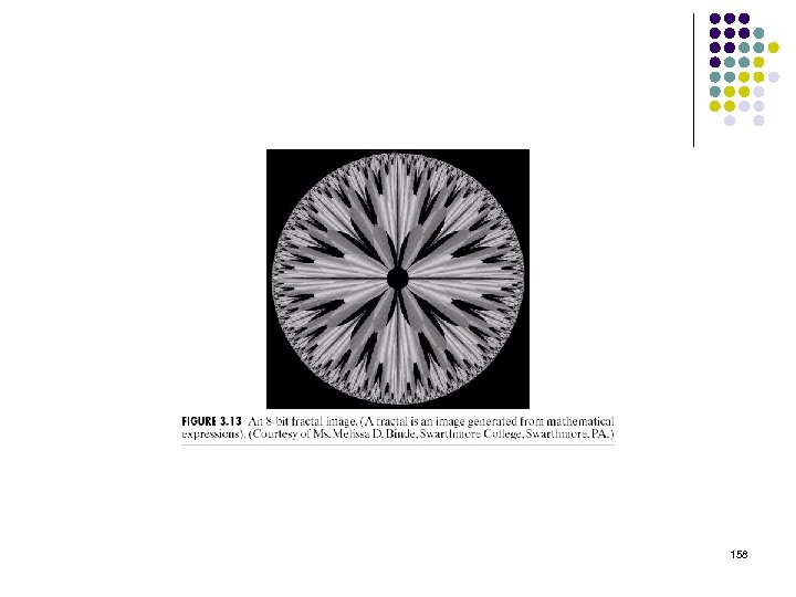
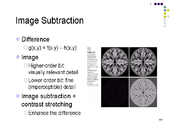
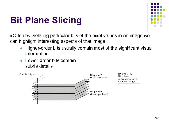 Bit Plane Slicing l. Often by isolating particular bits of the pixel values in an image we can highlight interesting aspects of that image l Higher-order bits usually contain most of the significant visual information l Lower-order bits contain subtle details 157
 158
158
![Bit Plane Slicing (cont…) [10000000] [01000000] [00100000] [00001000] [00000100] [00000001] 159 Bit Plane Slicing (cont…) [10000000] [01000000] [00100000] [00001000] [00000100] [00000001] 159](https://present5.com/presentation/b5707b29eab4372fb8188e5c594f81dd/image-159.jpg) Bit Plane Slicing (cont…) [10000000] [01000000] [00100000] [00001000] [00000100] [00000001] 159
Bit Plane Slicing (cont…) [10000000] [01000000] [00100000] [00001000] [00000100] [00000001] 159
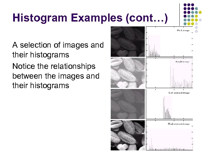 Histogram Examples (cont…) A selection of images and their histograms Notice the relationships between the images and their histograms 160
 161
161
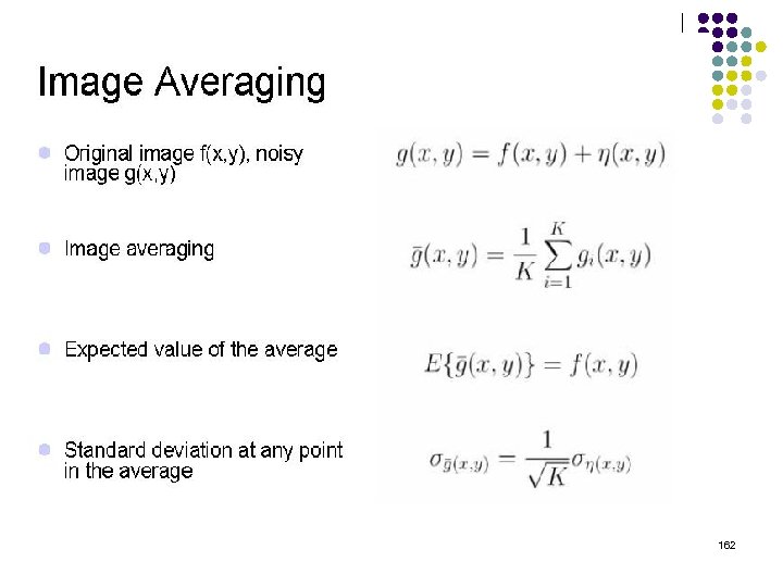 162
162
 163
163
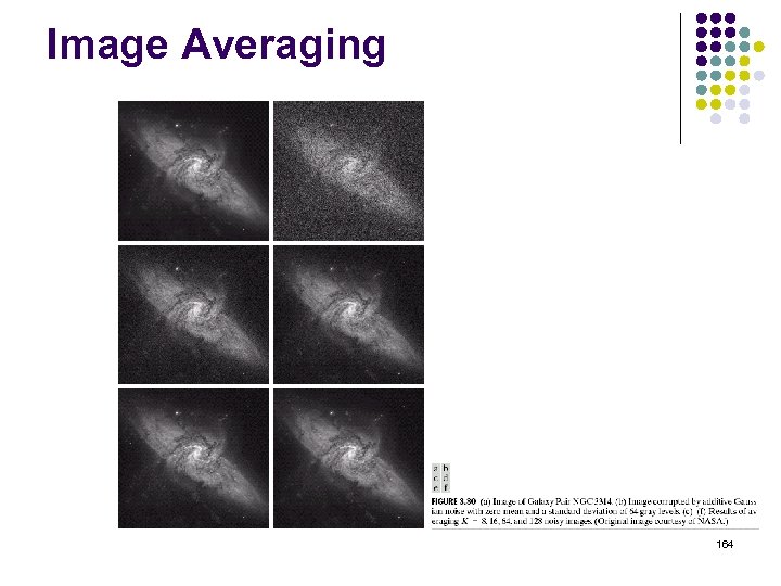 Image Averaging 164
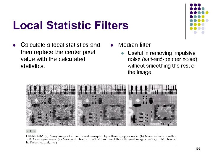 Local Statistic Filters l Calculate a local statistics and then replace the center pixel value with the calculated statistics. l Median filter l Useful in removing impulsive noise (salt-and-pepper noise) without smoothing the rest of the image. 165
 Sharpening Filters l To highlight fine detail or to enhance blurred detail. l l l smoothing ~ integration sharpening ~ differentiation Categories of sharpening filters: l l l Derivative operators Basic highpass spatial filtering High-boost filtering 166
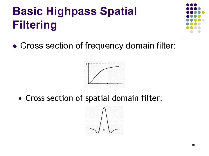 Basic Highpass Spatial Filtering l Cross section of frequency domain filter: • Cross section of spatial domain filter: 167
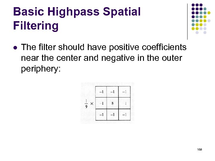 Basic Highpass Spatial Filtering l The filter should have positive coefficients near the center and negative in the outer periphery: 168
 Basic Highpass Spatial Filtering l The sum of the coefficients is 0, indicating that when the filter is passing over regions of almost stable gray levels, the output of the mask is 0 or very small. l Some scaling and/or clipping is involved (to compensate for possible negative gray levels after filtering). 169
 High-boost filter l High-boost or high-frequency-emphasis filter l Sharpens the image but does not remove the lowfrequency components unlike high-pass filtering 170
 High-boost filter l High-boost or high-frequency-emphasis filter l High pass = Original – Low pass l High boost = (A)(Original) - Low pass = (A-1) (Original) +Original – Lowpass = (A-1) (Original) + Highpass 171
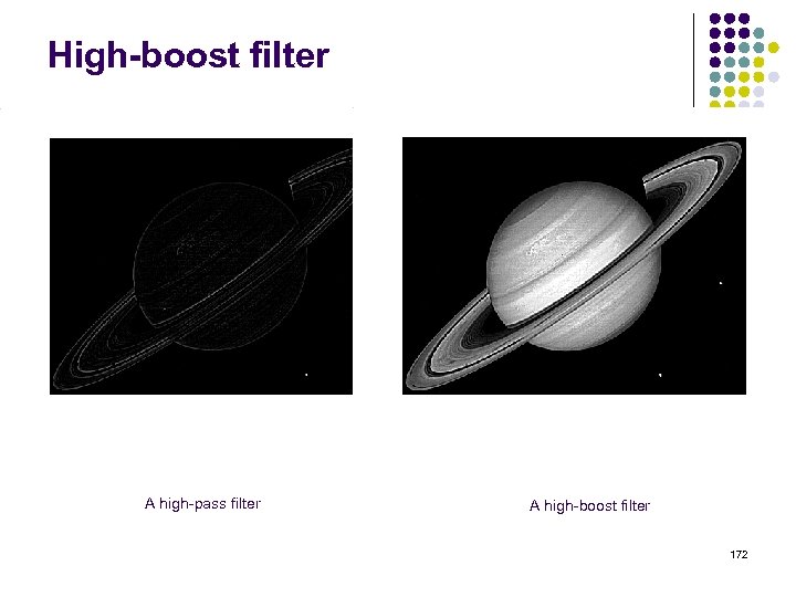 High-boost filter A high-pass filter A high-boost filter 172
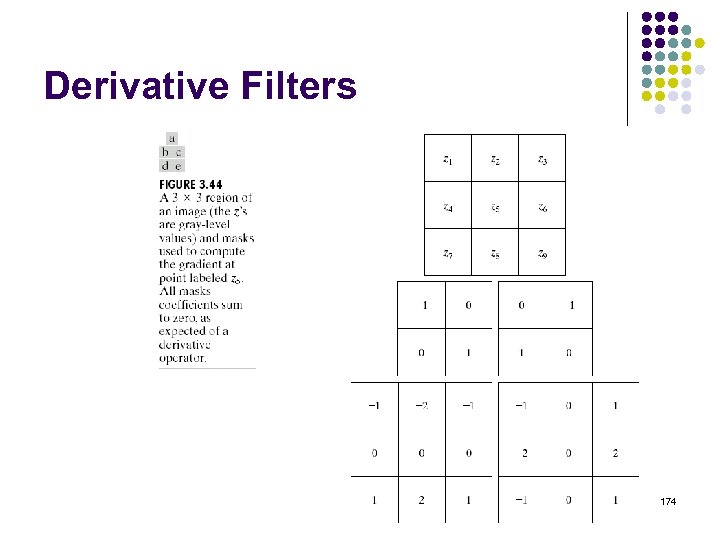
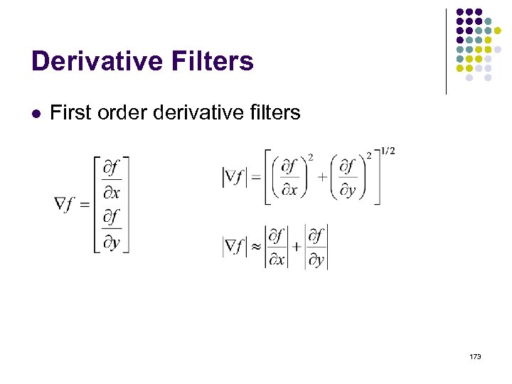 Derivative Filters l First order derivative filters 173
 Derivative Filters 174


