DEVOTED TO 210 -YEARS ANNIVERSARY OF KHARKIV NATIONAL

DEVOTED TO 210 -YEARS ANNIVERSARY OF KHARKIV NATIONAL MEDICAL UNIVERSITY MINISTRY OF PUBLIC HEALTH OF UKRAINE KHARKIV NATIONAL MEDICAL UNIVERSITY DEPARTMENT OF MEDICAL AND BIOLOGICAL PHYSICS AND MEDICAL INFORMATICS MEDICAL AND BIOLOGICAL PHYSICS Lectures KHARKIV - 2014

УДК 61: 53+577. 3](07. 07) ББК 28. 901 я 7 М 42 Approved by the Academic Council of Kharkiv National Medical University (minute N 5 at 22. 05. 2014) Reviewers: Berest V. P. - associate professor of Department of Molecular and Medical biophysics, Ph. D (Math. and Physics), V. N. Karazin Kharkiv National University Timanyuk V. O. - Chief of Department of Physics, professor, National University of Pharmacy Authors: Knigavko V. G. , Zaytseva O. V. , Batyuk L. V. , Bondarenko M. A M 42 Medical and Biological Physics. Lectures (in 2 parts): Textbook for students studying the subject in English: In 2 parts / Vladimir G. Knigavko, Olga V. Zaytseva, Lilia V. Batyuk, Marina A. Bondarenko. -Kharkiv: Kh. N. M. U. , 2014. ; Part I - 337 p. , Part II - 254 p. The Textbook covers the most important topics of medical and biological physics in compliance with the typical educational program. The structure and contents of the lectures completely correspond to credit-module system of educational process organization. The lectures are intended for teachers and students of the medical Universities, as well as for all interested in medical and biological physics. All rights reserved. No part of this publication may be reproduced in any material form (including photocopying or storing in any medium by electronic means and whether or not transiently or incidentally to some other use of this publication) without the written permission of the publishers. УДК 61: 53+577. 3](07. 07) ББК 28. 901 я 7 © Kharkiv National Medical University, 2014

Kharkiv National Medical University RANDOM VARIABLES Department of medical and biological physics and medical informatics

Plan of the lecture 1. Random variable (definition, types) 2. Discrete random variable; the distribution law; the condition of normalization 3. Continuous random variable; the probability density function; the condition of normalization; the distribution function 4. Numerical characteristic of random variable 5. Binomial distribution) (Bernoulli 6. Normal distribution) (Gauss

• A random variable is a variable quantity that randomly assumes a certain numerical value from a set of possible values resulting from a trial. • The occurrence of any value of this variable is a random event. • There are discrete and continuous random variables. • A random variable is called a discrete random variable if it has a finite or countable set of possible events. • For example, the number of students attending a lecture, the number of boys born at a maternity house in one day.

• To obtain a representation of a discrete random variable, it is necessary to specify the distribution law of this variable, i. e. enumerate all possible values of this variable and indicate the probabilities, which these values are assumed • The law of a discrete random variable distribution is shown in the following table: Values of X xi x 1 x 2 . . . xn Probabilities p(xi) p(x 1) p(x 2) . . . p(xn)

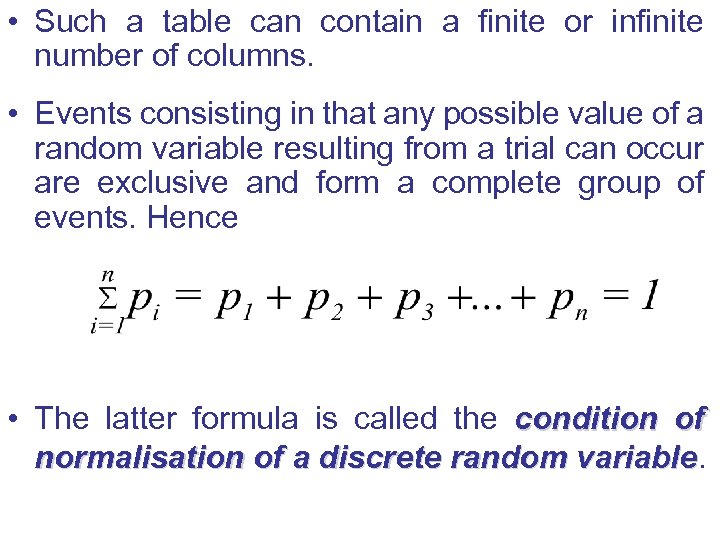• Such a table can contain a finite or infinite number of columns. • Events consisting in that any possible value of a random variable resulting from a trial can occur are exclusive and form a complete group of events. Hence • The latter formula is called the condition of normalisation of a discrete random variable

A continuous random variable is a random variable that can assume any value belonging to an interval (intervals) where it exists. For example, the temperature of a person, the duration of human life, the diameter of a pupil, the cardiac cycle duration and the blood sugar content are all examples of continuous random variables.

• Taking into account that a continuous random variable assumes an infinite set of values, the probability of the event that it will assume a certain concrete value equals zero. The probability of the zero. event that a continuous random variable will take a value from a certain interval is not equal to zero. • If we divide the domain of existence of a random variable to a number of intervals, and for each of these intervals define the probability of a random event falling therein, then the more intervals this domain would be divided to, the more precise the variable would be. • A continuous random variable would be defined most precisely if the interval dimensions tend to zero and the number of intervals tend to infinity.

The variable is equal to the ratio of the probability d. P of a random event falling in the interval from x to x+dx to the value of this interval dx is called the probability density function (or the frequency function) of a continuous random variable X, i. e. function where f(X) is the probability density function of a continuous random variable X. • Specifying the probability density function of a continuous random variable is one of the ways of defining this function (i. e. defining the law of distribution of this variable). From definition of f(X) it follows that the probability density function is a non-negative variable, i. e. f(X) 0.

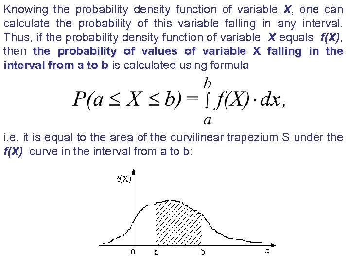Knowing the probability density function of variable X, one can calculate the probability of this variable falling in any interval. Thus, if the probability density function of variable X equals f(X), then the probability of values of variable X falling in the interval from a to b is calculated using formula i. e. it is equal to the area of the curvilinear trapezium S under the f(X) curve in the interval from a to b:

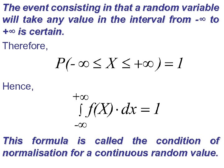The event consisting in that a random variable will take any value in the interval from -∞ to +∞ is certain. Therefore, Hence, This formula is called the condition of normalisation for a continuous random value.

To specify a continuous random variable, besides using the probability density, one can use the distribution function. The function distribution function F(X) of a continuous random variable X is related to the probability density f(X) of this random variable by the formulas

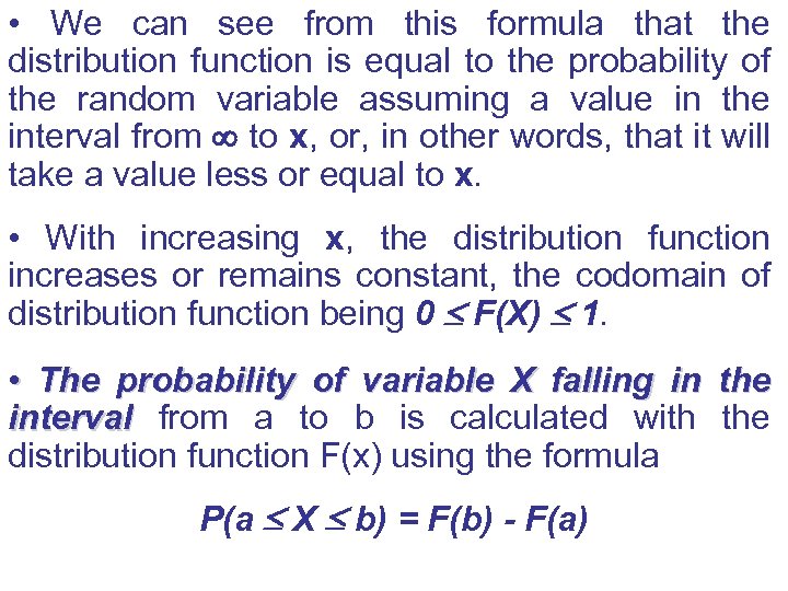• We can see from this formula that the distribution function is equal to the probability of the random variable assuming a value in the interval from tо x, or, in other words, that it will take a value less or equal to x. • With increasing x, the distribution function increases or remains constant, the codomain of distribution function being 0 F(X) 1. • The probability of variable X falling in the interval from a to b is calculated with the interval distribution function F(x) using the formula P(a X b) = F(b) - F(a)

Numeral Characteristics of Random Variables • Among the numeral characteristics of random variable X we shall consider three of them: mathematical expectation М(Х), variance D(X), standard deviation (Х).

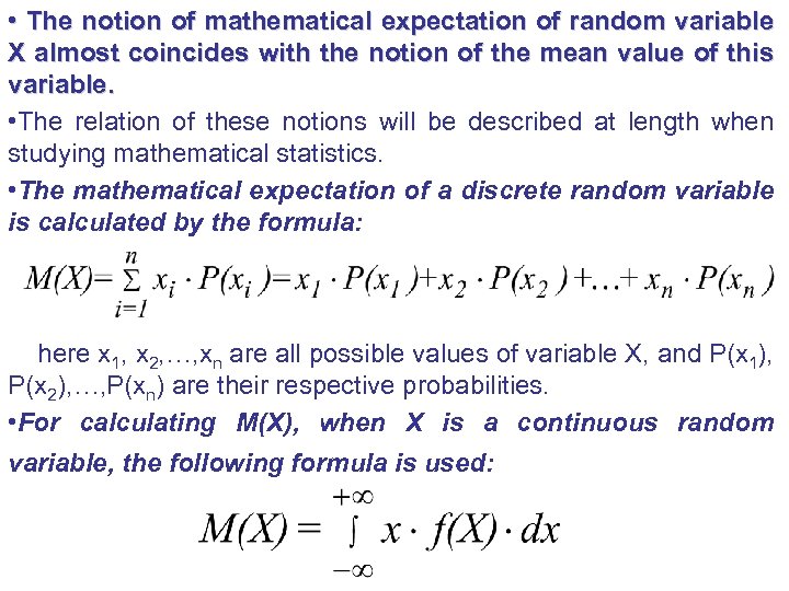• The notion of mathematical expectation of random variable X almost coincides with the notion of the mean value of this variable. • The relation of these notions will be described at length when studying mathematical statistics. • The mathematical expectation of a discrete random variable is calculated by the formula: here x 1, x 2, …, xn are all possible values of variable X, аnd P(x 1), P(x 2), …, P(xn) are their respective probabilities. • For calculating M(X), when X is a continuous random variable, the following formula is used:

• Variance and standard deviation characterise the magnitude of deviation (spread) of values of a random variable from its mathematical expectation. • Variance of random variable X is the mathematical expectation of the standard deviation of the values of this variable from its mathematical expectation, i. e. If X is a discrete random variable, its variance is found by the formula If X is a continuous random variable, the variance is found by the formula

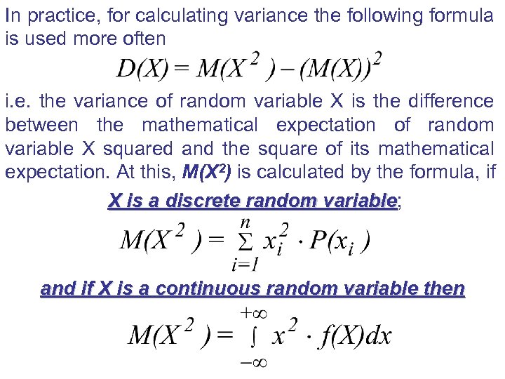In practice, for calculating variance the following formula is used more often i. e. the variance of random variable X is the difference between the mathematical expectation of random variable X squared and the square of its mathematical expectation. At this, M(X 2) is calculated by the formula, if X is a discrete random variable; variable and if X is a continuous random variable then

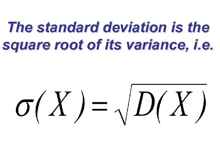The standard deviation is the square root of its variance, i. e.

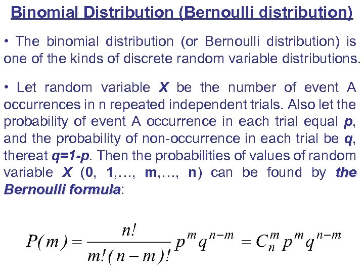Binomial Distribution (Bernoulli distribution) • The binomial distribution (or Bernoulli distribution) is one of the kinds of discrete random variable distributions. • Let random variable X be the number of event A occurrences in n repeated independent trials. Also let the probability of event A occurrence in each trial equal p, and the probability of non-occurrence in each trial be q, thereat q=1 -р. Then the probabilities of values of random variable Х (0, 1, …, m, …, n) can be found by the Bernoulli formula: formula

The right side of the Bernoulli formula is the common term of Newton's binomial expansion Therefore, the distribution of discrete random variable, wherein the probability of each value is equal to is called the law of binomial probability distribution The following table can present the distribution: Х Р(Х) 0 … … m … … n

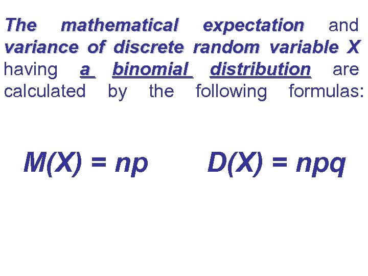The mathematical expectation and expectation variance of discrete random variable X having a binomial distribution are distribution calculated by the following formulas: М(Х) = np D(X) = npq

Normal Distribution (Gauss Distribution) The importance of studying the normal distribution is connected, in particular, with the fact that many variables, connected which characterise certain biological and medical objects, have distribution laws that are very close to the normal law. Such distribution laws are found in the following: - the height and weight of adults; - arterial blood pressure when examining a great number of patients; - the length of blood vessels; volume of organs; the weight and volume of brains found when performing anatomic examinations; - the absolute errors of readings of instruments, and measurement values; - the enzyme content in healthy people.

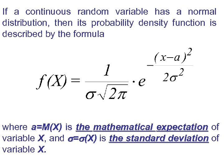If a continuous random variable has a normal distribution, then its probability density function is described by the formula where а=M(X) is the mathematical expectation of variable X, and = (X) is the standard deviation of variable X.

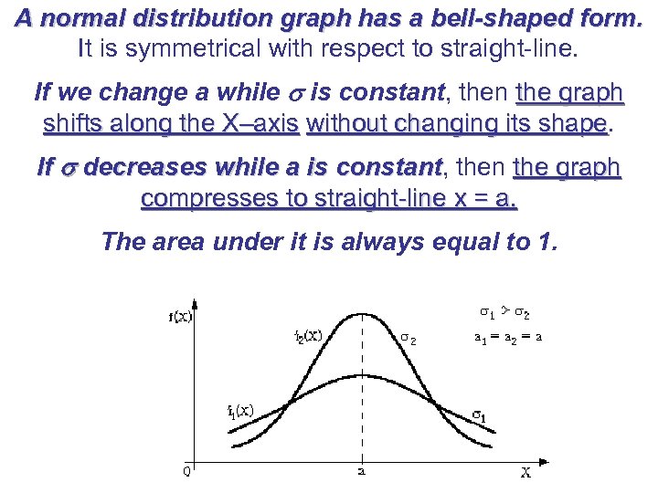A normal distribution graph has a bell-shaped form. It is symmetrical with respect to straight-line. If we change a while is constant, then the graph shifts along the X–axis without changing its shape If decreases while a is constant, then the graph constant compresses to straight-line х = а. The area under it is always equal to 1.

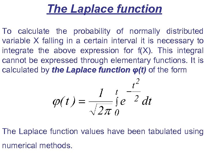The Laplace function To calculate the probability of normally distributed variable X falling in a certain interval it is necessary to integrate the above expression for f(X). This integral cannot be expressed through elementary functions. It is calculated by the Laplace function φ(t) of the form function The Laplace function values have been tabulated using numerical methods.

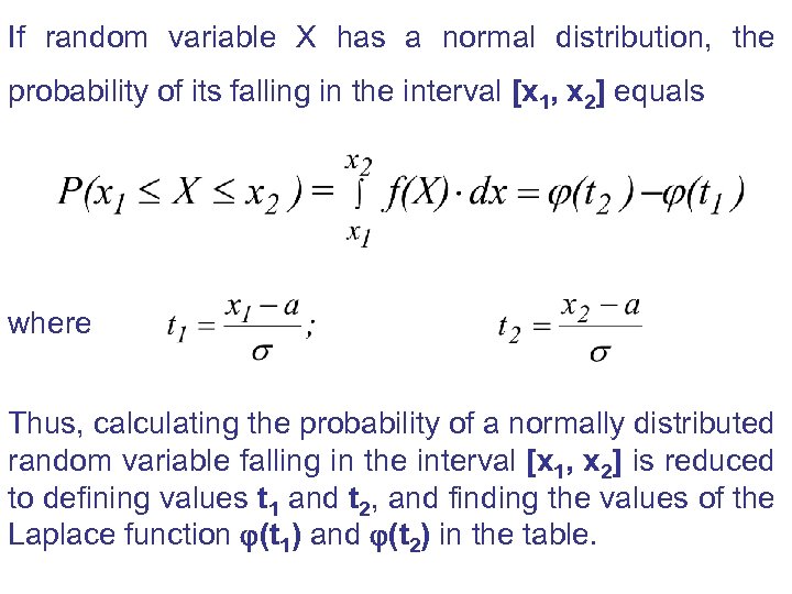If random variable X has a normal distribution, the probability of its falling in the interval [x 1, x 2] equals where Thus, calculating the probability of a normally distributed random variable falling in the interval [x 1, x 2] is reduced to defining values t 1 and t 2, and finding the values of the Laplace function (t 1) and (t 2) in the table.

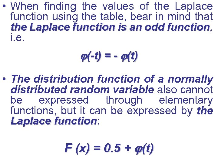• When finding the values of the Laplace function using the table, bear in mind that the Laplace function is an odd function, function i. e. (-t) = - (t) • The distribution function of a normally distributed random variable also cannot be expressed through elementary functions, but it can be expressed by the Laplace function: function F (x) = 0. 5 + (t)

Thank You for Attention!

Literature 1. Биофизика: учебник для вузов / П. Г. Костюк, Д. М. Гродзинський, В. Л. Зима и др. ; Под общ. ред. П. Г. Костюка. - К. : Вища шк. , 1988. - 504 с. 2. Биофизика / Ю. А. Владимиров, Д. И. Рощупкин, А. Я. Потапенко, А. И. Деев. – М. : Медицина, 1983. – 272 с. 3. Волькенштейн М. В. Биофизика. – М. : Наука, 1988. - 590 с. 4. Вибрационная безопасность. Общие требования. ГОСТ 12. 1. 012 -90. – М. , 1990. 5. Гамалея Н. Ф. , Рудых З. М. , Стадник В. Я. Лазеры в медицине. – К. : Здоровье, 1988. – 43 с. 6. Гродзинський Д. М. Радіобіологя. – К. : Либідь, 2000. – 448 с. 7. Губанов В. И. , Утепбергенов А. А. Медицинская биофизика. – М. : Медицина, 1978. – 336 с. 8. Ємчик Л. Ф. , Кміт Я. М. Медична і біологічна фізика. – Львів. : Світ, 2003. - 592 с. 9. Кольченко В. В. , Паничкин Ю. В. Ультразвук и сердце. – К. : Здоровья, 1988. – 45 с. 10. Кортуков Е. В. , Воеводский В. С. , Павлов Ю. К. Основы материаловедения. – М. : Высшая школа, 1988. – 322 с. 11. Котык А. , Яначек К. Мембранный транспорт. Междисциплинарный подход. – М. : Мир, 1980. – 341 с. 12. Луизов А. В. Физика зрения. – М. , Знание, 1976. – 62 с. 13. Маршелл Э. Биофизическая химия. Принципы, техника и приложения. В 2 -х томах. – М. : Мир, 1981. – 824 с. 14. Мэрион Дж. Общая физика с биологическими примерами. – М. : Высшая школа, 1986. – 623 с. 15. Медична і біологічна фзика. Том 1. / О. В. Чалий, Б. Т. Агапов, А. В. Меленевська та ін. – К. : ВІПОЛ, 1999. – 425 с. 16. Медична і біологічна фзика. Том 2. / О. В. Чалий, Б. Т. Агапов, А. В. Меленевська та ін. – К. : ВІПОЛ, 2001. – 415 с. 17. Проблемы прочности в биомеханике / И. Ф. Образцов, И. С. Адамович, А. С. Барер и др. – М. : Высшая школа, 1988. – 311 с. 18. Рего К. Г. Метрологическая обработка результатов технических измерений. – К. : Техніка, 1987. – 128 с. 19. Ремизов А. Н. Медицинская и биологическая физика. – М. : Высшая школа, 1999. – 616 с. 20. Рубин А. Б. Биофизика / Учеб. пособие для биол. спец. вузов. – М. : Высш. шк. , 1987. – 319 с. (1 том) 302 с (2 том) 21. Рубин А. Б. Термодинамика биологических процессов / Учеб. пособие для вузов. – М. : Изд-во МГУ, 1984. – 285 с. 22. Стенли А. Гельфанд. Слух: введение в психологическую и физиологическую акустику. – М. : Медицина, 1984. – 352 с. 23. Тиманюк В. А. , Животова Е. Н. Биофизика. – Харьков: Изд-во НФАУ; Золотые страницы, 2003. – 704 с. 24. Ультразвук. Маленькая энциклопедия. Глав. ред. И. П. Голямина. – М. : Советская Энциклопедия, 1979. – 400 с. 25. Ультразвук. Общие требования безопасности. ГОСТ 12. 1. 001 -89. – М. , 1989. 26. Физика визуализации изображений в медицине: В 2 -х т. Том 1; пер. с англ. /Под ред. С. Уэбба. – М. : Мир, 1991. – 408 с. 27. Физика визуализации изображений в медицине: В 2 -х т. Том 2; пер. с англ. /Под ред. С. Уэбба. – М. : Мир, 1991. – 423 с. 28. Фотометрия. Термины и определения. ГОСТ 26148 -84. – М. , 1984. 29. Хауссер К. Х. , Кальбитцер Х. Р. ЯМР в медицине и биологии: структура молекул, томография, спектроскопия in-vivo. – К. : Наук. Думка, 1993. – 259 с. 30. Холл Э. Дж. Радиация и жизнь. – М. : Медицина, 1989. – 256 с. 31. Шандала М. Г. , Думанский Ю. Д. , Иванов Д. С. Санитарный надзор за источниками электромагнитных излучений в окружающей среде. – К. : Здоровье, 1990. – 150 с. 32. Шум. Допустимые уровни в жилых и общественных зданиях. ГОСТ 12. 1. 036 -81. – М. , 1981. 33. Электростатические поля. Допустимые уровни на рабочих местах и требовании к проведению контроля. ГОСТ 12. 1. 045 -84. – М. , 1984. 34. Ярмоненко С. П. Радиобиология человека и животных. - М. : Высшая школа, 1988. – 423 с.