Determining Optimal Level of Product Availability 1

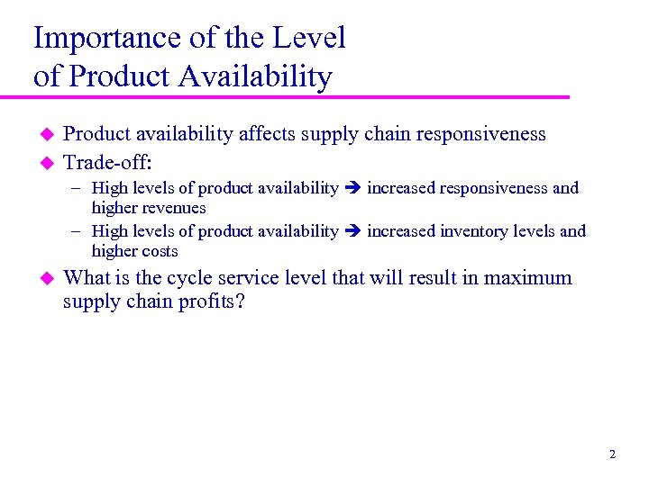
Importance of the Level of Product Availability u u Product availability affects supply chain responsiveness Trade-off: – High levels of product availability increased responsiveness and higher revenues – High levels of product availability increased inventory levels and higher costs u What is the cycle service level that will result in maximum supply chain profits? 2

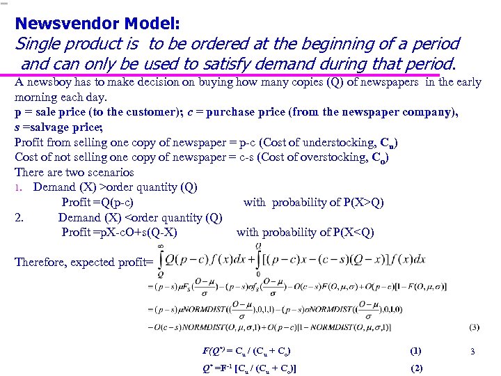
Newsvendor Model: Single product is to be ordered at the beginning of a period and can only be used to satisfy demand during that period. A newsboy has to make decision on buying how many copies (Q) of newspapers in the early morning each day. p = sale price (to the customer); c = purchase price (from the newspaper company), s =salvage price; Profit from selling one copy of newspaper = p-c (Cost of understocking, Cu) Cost of not selling one copy of newspaper = c-s (Cost of overstocking, Co) There are two scenarios 1. Demand (X) >order quantity (Q) Profit =Q(p-c) with probability of P(X>Q) 2. Demand (X) <order quantity (Q) Profit =p. X-c. O+s(Q-X) with probability of P(X<Q) Therefore, expected profit= F(Q*) = Cu / (Cu + Co) (1) Q* =F-1 [Cu / (Cu + Co)] (2) 3

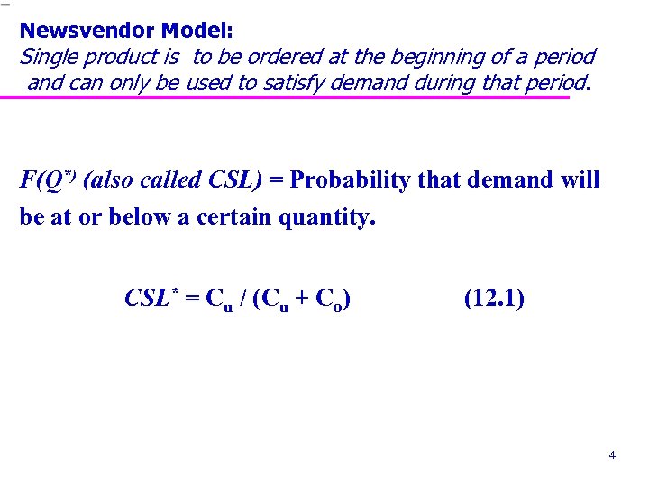
Newsvendor Model: Single product is to be ordered at the beginning of a period and can only be used to satisfy demand during that period. F(Q*) (also called CSL) = Probability that demand will be at or below a certain quantity. CSL* = Cu / (Cu + Co) (12. 1) 4

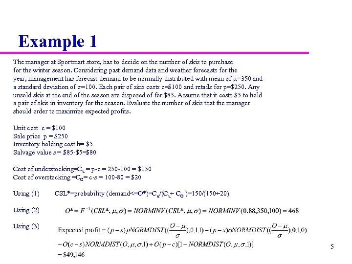
Example 1 The manager at Sportmart store, has to decide on the number of skis to purchase for the winter season. Considering past demand data and weather forecasts for the year, management has forecast demand to be normally distributed with mean of µ=350 and a standard deviation of σ=100. Each pair of skis costs c=$100 and retails for p=$250. Any unsold skis at the end of the season are disposed of for $85. Assume that it costs $5 to hold a pair of skis in inventory for the season. Evaluate the number of skis that the manager should order to maximize expected profits. Unit cost c = $100 Sale price p = $250 Inventory holding cost h= $5 Salvage value s = $85 -$5=$80 Cost of understocking=Cu = p-c = 250 -100 = $150 Cost of overstocking =CO= c-s = 100 -80 = $20 Using (1) CSL*=probability (demand<=O*)=Cu/(Cu+ CO )=150/(150+20) Using (2) Using (3) 5

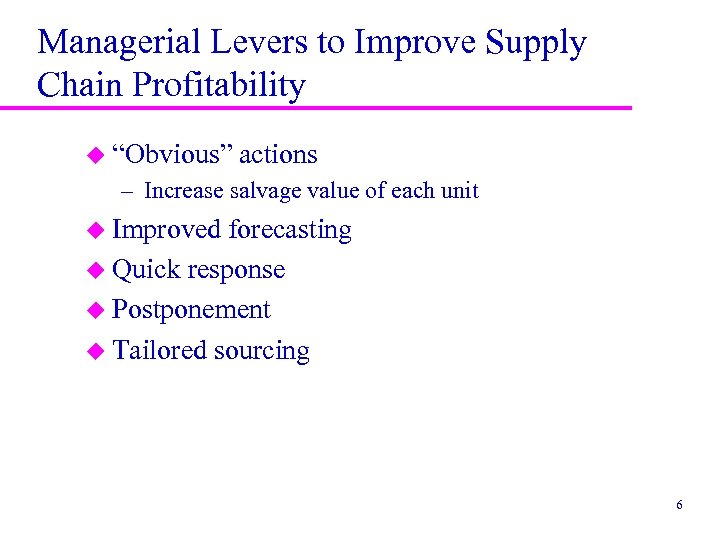
Managerial Levers to Improve Supply Chain Profitability u “Obvious” actions – Increase salvage value of each unit u Improved forecasting u Quick response u Postponement u Tailored sourcing 6

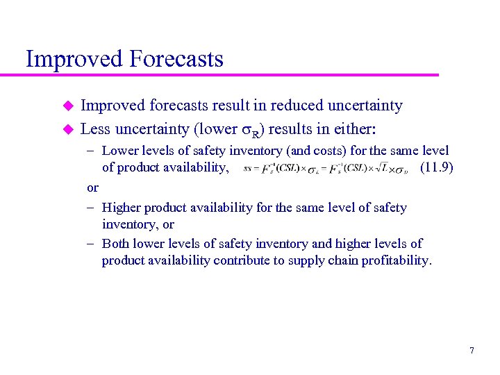
Improved Forecasts u u Improved forecasts result in reduced uncertainty Less uncertainty (lower R) results in either: – Lower levels of safety inventory (and costs) for the same level of product availability, (11. 9) or – Higher product availability for the same level of safety inventory, or – Both lower levels of safety inventory and higher levels of product availability contribute to supply chain profitability. 7

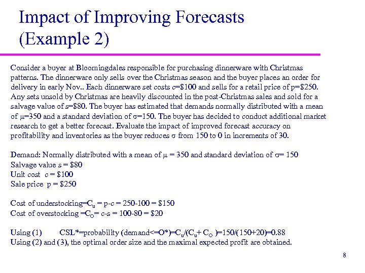
Impact of Improving Forecasts (Example 2) Consider a buyer at Bloomingdales responsible for purchasing dinnerware with Christmas patterns. The dinnerware only sells over the Christmas season and the buyer places an order for delivery in early Nov. . Each dinnerware set costs c=$100 and sells for a retail price of p=$250. Any sets unsold by Christmas are heavily discounted in the post-Christmas sales and sold for a salvage value of s=$80. The buyer has estimated that demands normally distributed with a mean of µ=350 and a standard deviation of σ=150. The buyer has decided to conduct additional market research to get a better forecast. Evaluate the impact of improved forecast accuracy on profitability and inventories as the buyer reduces σ from 150 to 0 in increments of 30. Demand: Normally distributed with a mean of µ = 350 and standard deviation of = 150 Salvage value s = $80 Unit cost c = $100 Sale price p = $250 Cost of understocking=Cu = p-c = 250 -100 = $150 Cost of overstocking =CO= c-s = 100 -80 = $20 Using (1) CSL*=probability (demand<=O*)=Cu/(Cu+ CO )=150/(150+20)=0. 88 Using (2) and (3), the optimal order size and the maximal expected profit are obtained. 8

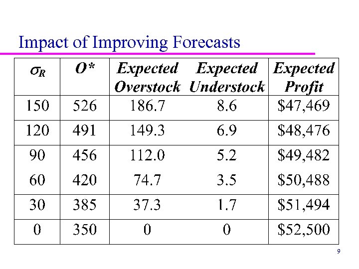
Impact of Improving Forecasts 9

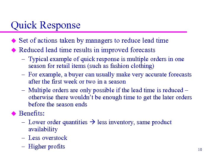
Quick Response u u Set of actions taken by managers to reduce lead time Reduced lead time results in improved forecasts – Typical example of quick response is multiple orders in one season for retail items (such as fashion clothing) – For example, a buyer can usually make very accurate forecasts after the first week or two in a season – Multiple orders are only possible if the lead time is reduced – otherwise there wouldn’t be enough time to get the later orders before the season ends u Benefits: – Lower order quantities less inventory, same product availability – Less overstock – Higher profits 10

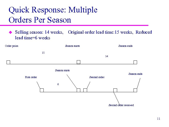
Quick Response: Multiple Orders Per Season u Selling season: 14 weeks, lead time=6 weeks Order point Original order lead time: 15 weeks, Reduced Season starts Season ends 15 14 Season starts Season ends First order Second order 6 Second order received 11

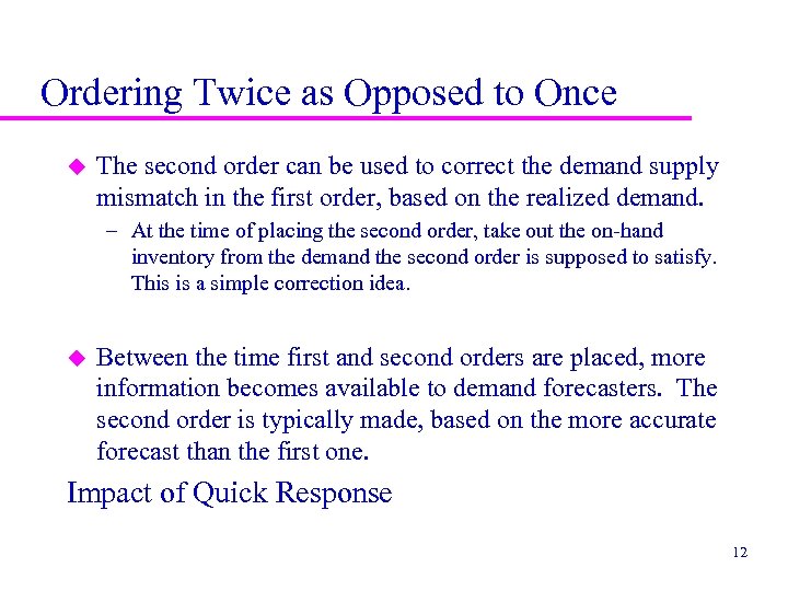
Ordering Twice as Opposed to Once u The second order can be used to correct the demand supply mismatch in the first order, based on the realized demand. – At the time of placing the second order, take out the on-hand inventory from the demand the second order is supposed to satisfy. This is a simple correction idea. u Between the time first and second orders are placed, more information becomes available to demand forecasters. The second order is typically made, based on the more accurate forecast than the first one. Impact of Quick Response 12

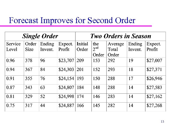
Forecast Improves for Second Order 13

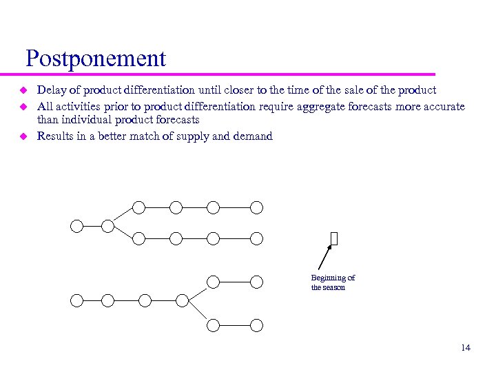
Postponement u u u Delay of product differentiation until closer to the time of the sale of the product All activities prior to product differentiation require aggregate forecasts more accurate than individual product forecasts Results in a better match of supply and demand Beginning of the season 14

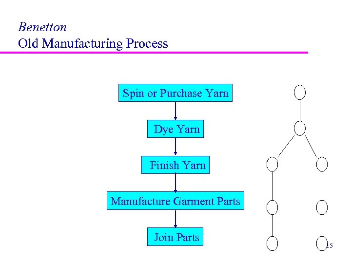
Benetton Old Manufacturing Process Spin or Purchase Yarn Dye Yarn Finish Yarn Manufacture Garment Parts Join Parts 15

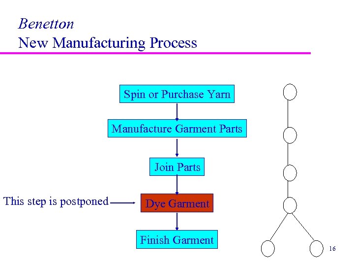
Benetton New Manufacturing Process Spin or Purchase Yarn Manufacture Garment Parts Join Parts This step is postponed Dye Garment Finish Garment 16

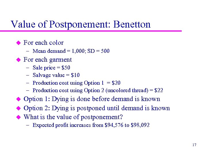
Value of Postponement: Benetton u For each color – Mean demand = 1, 000; SD = 500 u For each garment – – u u u Sale price = $50 Salvage value = $10 Production cost using Option 1 = $20 Production cost using Option 2 (uncolored thread) = $22 Option 1: Dying is done before demand is known Option 2: Dying is postponed until demand is known What is the value of postponement? – Expected profit increases from $94, 576 to $98, 092 17

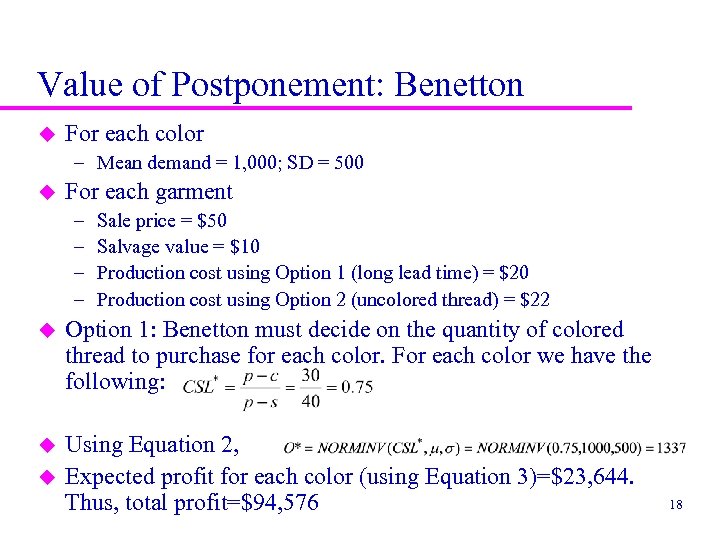
Value of Postponement: Benetton u For each color – Mean demand = 1, 000; SD = 500 u For each garment – – Sale price = $50 Salvage value = $10 Production cost using Option 1 (long lead time) = $20 Production cost using Option 2 (uncolored thread) = $22 u Option 1: Benetton must decide on the quantity of colored thread to purchase for each color. For each color we have the following: u Using Equation 2, Expected profit for each color (using Equation 3)=$23, 644. Thus, total profit=$94, 576 u 18

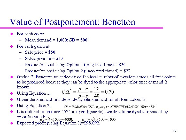
Value of Postponement: Benetton u u u u For each color – Mean demand = 1, 000; SD = 500 For each garment – Sale price = $50 – Salvage value = $10 – Production cost using Option 1 (long lead time) = $20 – Production cost using Option 2 (uncolored thread) = $22 Option 2: Benetton must decide on the total number of sweaters across all four colors to be produced because they can be dyed to the appropriate color once demand is known. Using Equation 1, Given that demand in independent, total demand for all four colors is Using Equation 2, It is optimal to produce 4524 undyed (generic) sweaters to be dyed as demand by color is available. Expected profit (using Equation 3)=$98. 092. 19

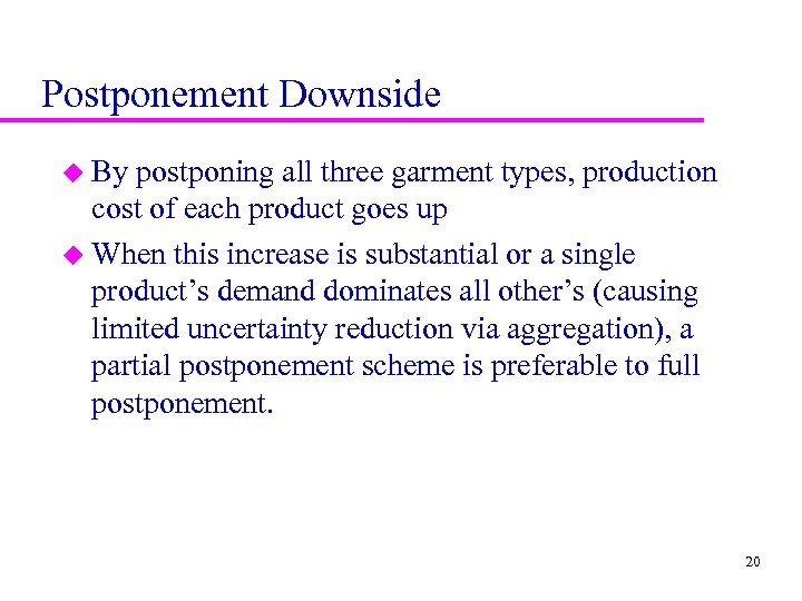
Postponement Downside u By postponing all three garment types, production cost of each product goes up u When this increase is substantial or a single product’s demand dominates all other’s (causing limited uncertainty reduction via aggregation), a partial postponement scheme is preferable to full postponement. 20

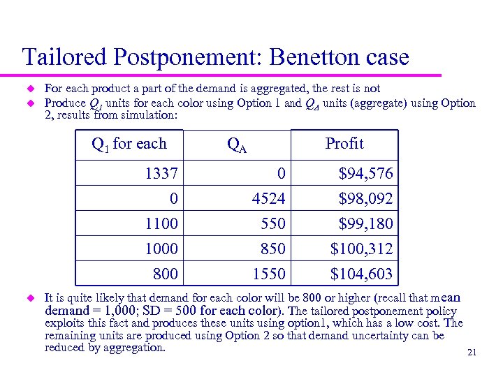
Tailored Postponement: Benetton case u u For each product a part of the demand is aggregated, the rest is not Produce Q 1 units for each color using Option 1 and QA units (aggregate) using Option 2, results from simulation: Q 1 for each QA Profit 1337 0 1100 $94, 576 $98, 092 $99, 180 1000 800 u 0 4524 550 850 1550 $100, 312 $104, 603 It is quite likely that demand for each color will be 800 or higher (recall that mean demand = 1, 000; SD = 500 for each color). The tailored postponement policy exploits this fact and produces these units using option 1, which has a low cost. The remaining units are produced using Option 2 so that demand uncertainty can be reduced by aggregation. 21

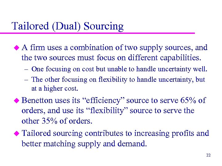
Tailored (Dual) Sourcing u. A firm uses a combination of two supply sources, and the two sources must focus on different capabilities. – One focusing on cost but unable to handle uncertainty well. – The other focusing on flexibility to handle uncertainty, but at a higher cost. u Benetton uses its “efficiency” source to serve 65% of orders, and use its “flexibility” source to serve the other 35% of orders. u Tailored sourcing contributes to increasing profits and better matching supply and demand. 22

Supply Chain Contracts and Their Impact on Profitability u Returns policy: Buyback contracts u Revenue sharing contract. u Vendor-managed inventories 23

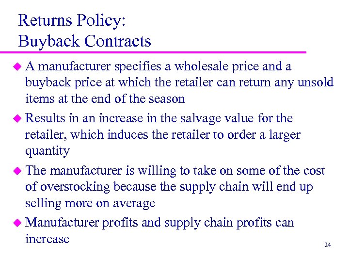
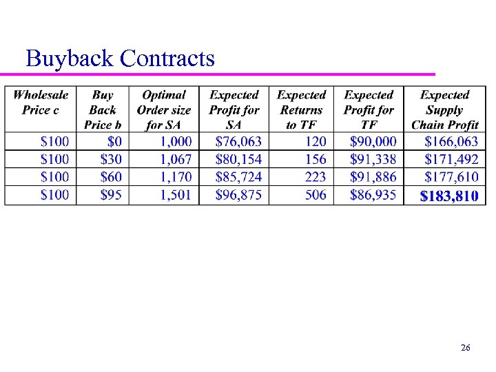
Returns Policy: Buyback Contracts u. A manufacturer specifies a wholesale price and a buyback price at which the retailer can return any unsold items at the end of the season u Results in an increase in the salvage value for the retailer, which induces the retailer to order a larger quantity u The manufacturer is willing to take on some of the cost of overstocking because the supply chain will end up selling more on average u Manufacturer profits and supply chain profits can increase 24

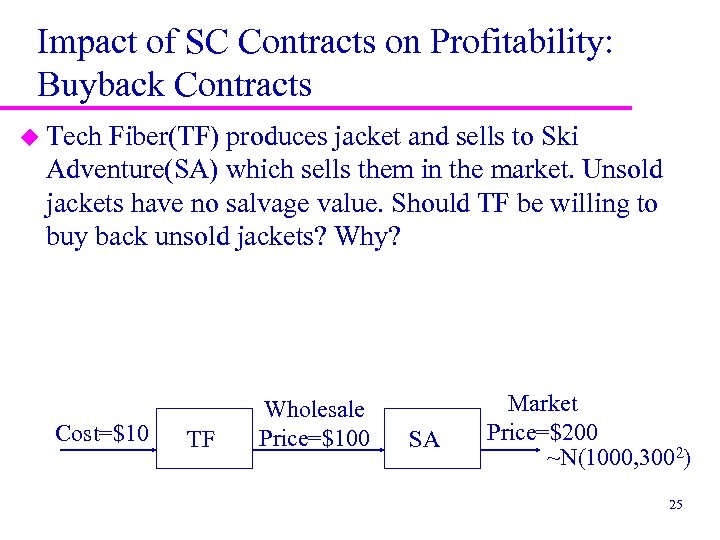
Impact of SC Contracts on Profitability: Buyback Contracts u Tech Fiber(TF) produces jacket and sells to Ski Adventure(SA) which sells them in the market. Unsold jackets have no salvage value. Should TF be willing to buy back unsold jackets? Why? Cost=$10 TF Wholesale Price=$100 SA Market Price=$200 ~N(1000, 3002) 25

Buyback Contracts 26

Revenue Sharing Contracts u u The manufacturer charges the retailer a low (or even zero) wholesale price and shares a fraction of the revenue generated by the retailer The lower wholesale price decreases the cost to the retailer in case of an overstock The retailer therefore increases the level of product availability, which results in higher profits for both the manufacturer and the retailer The impact of revenue sharing on Blockbuster was dramatic – Rentals increased by 75% in test markets – Market share increased from 25% to 31% (The 2 nd largest retailer, Hollywood Entertainment Corp has 5% market share) 27

Traditional Situation Selling Price=$200 Wholesale Price =$100 Manufacturer DC Salvage Value=$0 Demand ~N (1000, 3002) Retail DC Production cost=$10 Stores 28

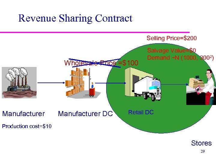
Revenue Sharing Contract Selling Price=$200 Wholesale Price =$100 Manufacturer DC Salvage Value=$0 Demand ~N (1000, 3002) Retail DC Production cost=$10 Stores 29

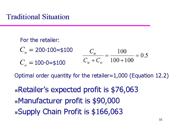
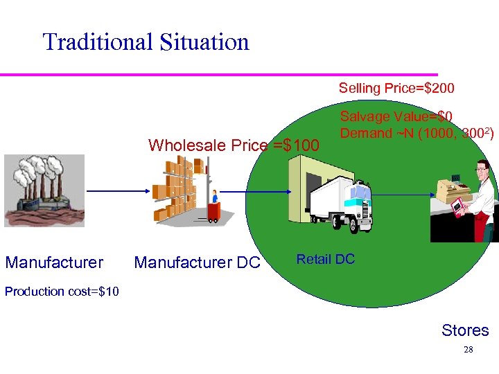
Traditional Situation For the retailer: 200 -100=$100 100 -0=$100 Optimal order quantity for the retailer=1, 000 (Equation 12. 2) Retailer’s expected profit is $76, 063 n. Manufacturer profit is $90, 000 n. Supply Chain Profit is $166, 063 n 30

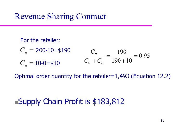
Revenue Sharing Contract For the retailer: 200 -10=$190 10 -0=$10 Optimal order quantity for the retailer=1, 493 (Equation 12. 2) n Supply Chain Profit is $183, 812 31

Vendor-Managed Inventories (VMI) u u Manufacturer or supplier is responsible for all decisions regarding inventory at the retailer Control of replenishment decisions moves to the manufacturer Requires that the retailer share demand information with the manufacturer Having final customer demand data also helps manufacturer plan production more effectively, at the same time it enables the manufacturer to respond to the retailer more quickly appropriately scheduling production and replenishing the retailer inventory. 32

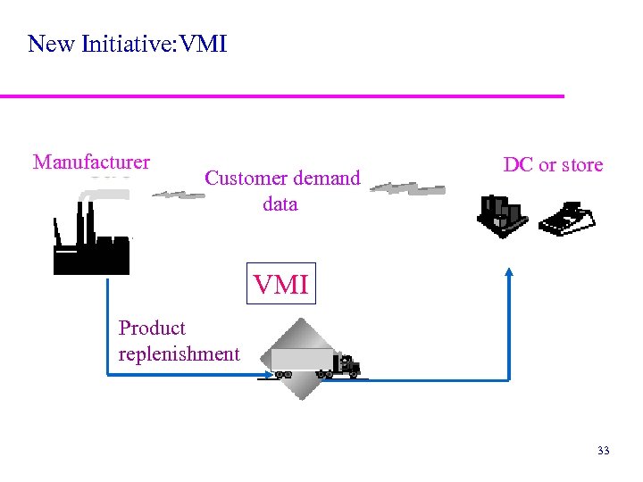
New Initiative: VMI Manufacturer Customer demand data DC or store VMI Product replenishment 33