Determinants of the House Bidding Process Approximating the

Determinants of the House Bidding Process: Approximating the Seller’s Surplus? Sotirios Thanos, David Watkins, & Michael White Heriot-Watt University, Edinburgh

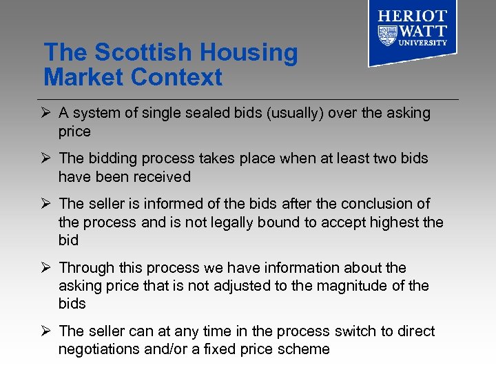
The Scottish Housing Market Context Ø A system of single sealed bids (usually) over the asking price Ø The bidding process takes place when at least two bids have been received Ø The seller is informed of the bids after the conclusion of the process and is not legally bound to accept highest the bid Ø Through this process we have information about the asking price that is not adjusted to the magnitude of the bids Ø The seller can at any time in the process switch to direct negotiations and/or a fixed price scheme

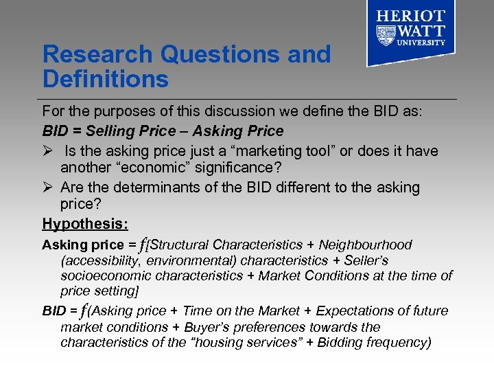
Research Questions and Definitions For the purposes of this discussion we define the BID as: BID = Selling Price – Asking Price Ø Is the asking price just a “marketing tool” or does it have another “economic” significance? Ø Are the determinants of the BID different to the asking price? Hypothesis: Asking price = f[Structural Characteristics + Neighbourhood (accessibility, environmental) characteristics + Seller’s socioeconomic characteristics + Market Conditions at the time of price setting] BID = f(Asking price + Time on the Market + Expectations of future market conditions + Buyer’s preferences towards the characteristics of the “housing services” + Bidding frequency)

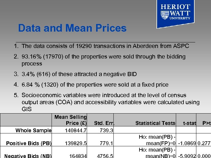
Data and Mean Prices 1. The data consists of 19290 transactions in Aberdeen from ASPC 2. 93. 16% (17970) of the properties were sold through the bidding process 3. 3. 4% (616) of these attracted a negative BID 4. 6. 84 % (1320) of the properties were sold at a fixed price 5. Socioeconomic variables were introduced at the level of census output areas (COA) and accessibility variables were calculated using GIS Mean Selling Table 1: Mean Selling Price (£) Whole Sample 140844. 7 Std. Err. 739. 3 Positive Bids (PB) 139829. 5 779. 1 Negative Bids (NB) 164834 4756. 5 Statistical Tests t-stat P>t Ho: mean(PB) - mean(FP)=0 -1. 0869 0. 277 Ho: mean(PB) - mean(NB)=0 -5. 9092 0. 000

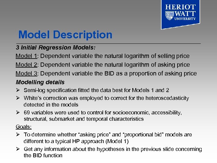
Model Description 3 Initial Regression Models: Model 1: Dependent variable the natural logarithm of selling price Model 2: Dependent variable the natural logarithm of asking price Model 3: Dependent variable the BID as a proportion of asking price Modelling details Ø Semi-log specification fitted the data best for Models 1 and 2 Ø White’s correction was employed to correct for the heteroscedasticity detected in the models Ø 69 variables were used to control for socioeconomic, accessibility, structural, submarket and temporal characteristics Goals: Ø To determine whether “asking price” and “proportional bid” models are different to a typical HP approach (Model 1) Ø Get any information about the hypotheses in the previous slide concerning the BID function

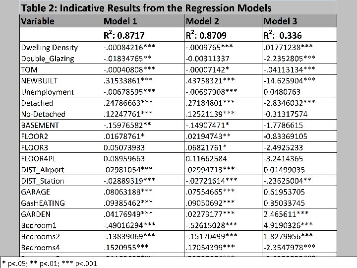
* p<. 05; ** p<. 01; *** p<. 001

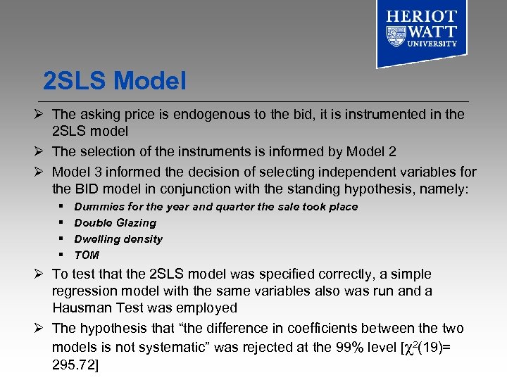
2 SLS Model Ø The asking price is endogenous to the bid, it is instrumented in the 2 SLS model Ø The selection of the instruments is informed by Model 2 Ø Model 3 informed the decision of selecting independent variables for the BID model in conjunction with the standing hypothesis, namely: § § Dummies for the year and quarter the sale took place Double Glazing Dwelling density TOM Ø To test that the 2 SLS model was specified correctly, a simple regression model with the same variables also was run and a Hausman Test was employed Ø The hypothesis that “the difference in coefficients between the two models is not systematic” was rejected at the 99% level [χ2(19)= 295. 72]

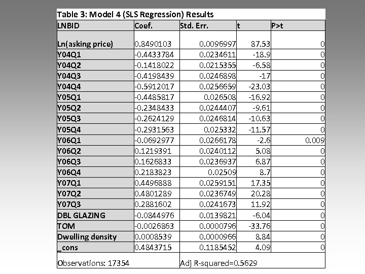
Table 3: Model 4 (SLS Regression) Results LNBID Coef. Ln(asking price) Y 04 Q 1 Y 04 Q 2 Y 04 Q 3 Y 04 Q 4 Y 05 Q 1 Y 05 Q 2 Y 05 Q 3 Y 05 Q 4 Y 06 Q 1 Y 06 Q 2 Y 06 Q 3 Y 06 Q 4 Y 07 Q 1 Y 07 Q 2 Y 07 Q 3 DBL GLAZING TOM Dwelling density _cons 0. 8490103 -0. 4433784 -0. 1418022 -0. 4198439 -0. 5912017 -0. 4485817 -0. 2348433 -0. 2624129 -0. 2931563 -0. 0692977 0. 1219391 0. 1626833 0. 2183823 0. 4496888 0. 4801289 0. 2881602 -0. 0844976 -0. 0026863 0. 0008539 0. 4843715 Observations: 17354 Std. Err. 0. 0096997 0. 0234611 0. 0215355 0. 0246898 0. 0256659 0. 026508 0. 0244407 0. 0246814 0. 025332 0. 0266178 0. 0240112 0. 0236937 0. 02509 0. 0259151 0. 0236749 0. 0241673 0. 0139821 0. 0000796 0. 0000966 0. 1185452 t P>t 87. 53 -18. 9 -6. 58 -17 -23. 03 -16. 92 -9. 61 -10. 63 -11. 57 -2. 6 5. 08 6. 87 8. 7 17. 35 20. 28 11. 92 -6. 04 -33. 76 8. 84 4. 09 Adj R-squared=0. 5629 0 0 0 0 0. 009 0 0 0 0 0

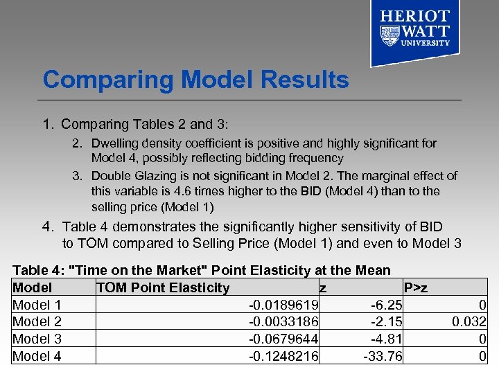
Comparing Model Results 1. Comparing Tables 2 and 3: 2. Dwelling density coefficient is positive and highly significant for Model 4, possibly reflecting bidding frequency 3. Double Glazing is not significant in Model 2. The marginal effect of this variable is 4. 6 times higher to the BID (Model 4) than to the selling price (Model 1) 4. Table 4 demonstrates the significantly higher sensitivity of BID to TOM compared to Selling Price (Model 1) and even to Model 3 Table 4: "Time on the Market" Point Elasticity at the Mean Model TOM Point Elasticity z P>z Model 1 -0. 0189619 -6. 25 Model 2 -0. 0033186 -2. 15 Model 3 -0. 0679644 -4. 81 Model 4 -0. 1248216 -33. 76 0 0. 032 0 0

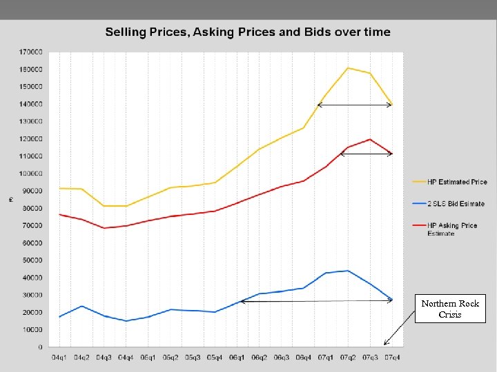
Northern Rock Crisis

Discussion Ø The BID may depend on environmental preferences, as the double glazing variable might have indicated Ø As expected TOM is a strong determinant of the BID Ø TOM has been found in the literature to depend upon market conditions (e. g. Pryce and Gibb, 2006) Ø We have found that the BID is also highly dependent on market conditions, reflecting buyer expectations for future market movements Ø The asking price could be interpreted as a signal of the sellers reserve price to the buyer. Hence, the BID could operate as a proxy to the seller’s surplus. Ø Some weak evidence of a time lag by which the asking price is adjusted to previous bidding processes (witnessed by real estate agents / solicitors)

Further Research Ø Logit models to address the choice of selling method (fixed price or bidding) is one research avenue. Ø Stated preference experiments might also prove enlightening with regard to this question Ø Noise measurements will be included in the models, determining whether the purchaser’s environmental preferences are reflected in the BID Ø We recognise that the treatment of TOM is simplistic here and a more “state of the art” approach is the next step

THANK YOU