Design evaluation and optimization for models of hepatitis

Design evaluation and optimization for models of hepatitis C viral dynamics Jeremie Guedj 1, 2 Caroline Bazzoli 3 Avidan Neumann 2 France Mentré 3 1 Los Alamos National Laboratory, New Mexico, USA. 2 Bar-Ilan University, Ramat-Gan, Israel. 3 UMR 738 INSERM and University Paris Diderot, Paris, France. 1

Background (1) Chronic hepatitis C virus (HCV) infection is one of the most common causes of chronic liver disease, with as many as 170 million people infected worldwide n The standard of care is weekly injections of pegylated interferon + daily oral ribavirin n After a year treatment viral eradication is achieved in 50% in HCV genotype 1 patients n 2

Background (2) Mathematical modeling of HCV RNA (viral load) decay after treatment initiation has brought critical insights for the understanding of the virus pathogenesis n The parameters of this model are crucial for early predicting treatment outcome (

Modeling HCV RNA decay with daily IFN T 0 Neumann et al. (Science 1998) (1 -h)b infection I V c clearance (1 -ep)p production d death / loss Target cells (T), infected cells (I) and free virus (V) 4

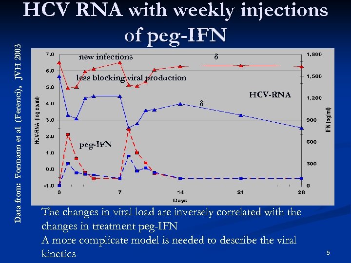Data from: Formann et al (Ferenci), JVH 2003 HCV RNA with weekly injections of peg-IFN new infections δ less blocking viral production δ HCV-RNA peg-IFN The changes in viral load are inversely correlated with the changes in treatment peg-IFN A more complicate model is needed to describe the viral kinetics 5

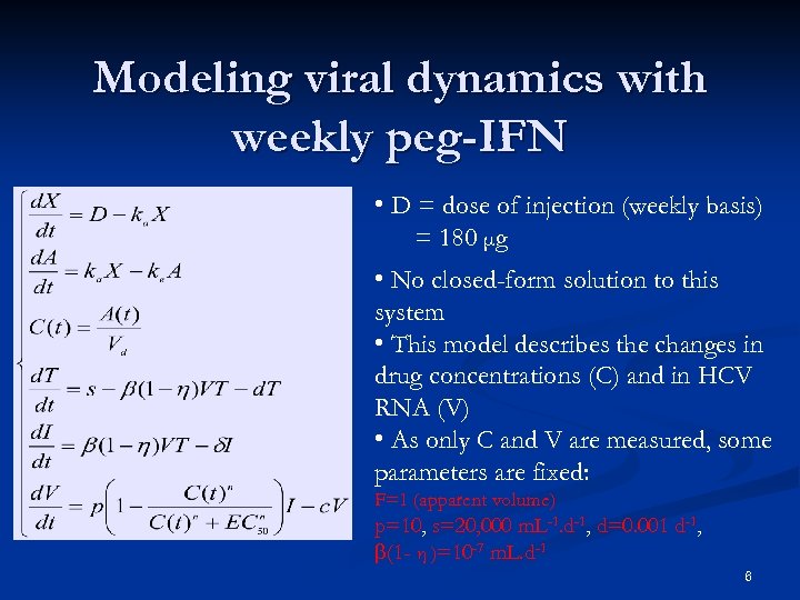Modeling viral dynamics with weekly peg-IFN • D = dose of injection (weekly basis) = 180 μg • No closed-form solution to this system • This model describes the changes in drug concentrations (C) and in HCV RNA (V) • As only C and V are measured, some parameters are fixed: F=1 (apparent volume) p=10, s=20, 000 m. L-1. d-1, d=0. 001 d-1, b(1 - η )=10 -7 m. L. d-1 6

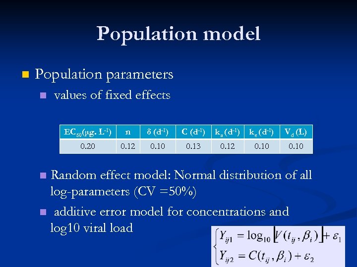Population model n Population parameters n values of fixed effects EC 50(μg. L-1) n δ (d-1) C (d-1) ka (d-1) ke (d-1) Vd (L) 0. 20 0. 12 0. 10 0. 13 0. 12 0. 10 Random effect model: Normal distribution of all log-parameters (CV =50%) n additive error model for concentrations and log 10 viral load n

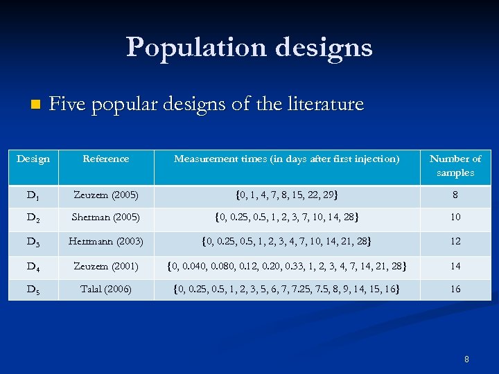Population designs n Five popular designs of the literature Design Reference Measurement times (in days after first injection) Number of samples D 1 Zeuzem (2005) {0, 1, 4, 7, 8, 15, 22, 29} 8 D 2 Sherman (2005) {0, 0. 25, 0. 5, 1, 2, 3, 7, 10, 14, 28} 10 D 3 Herrmann (2003) {0, 0. 25, 0. 5, 1, 2, 3, 4, 7, 10, 14, 21, 28} 12 D 4 Zeuzem (2001) {0, 0. 040, 0. 080, 0. 12, 0. 20, 0. 33, 1, 2, 3, 4, 7, 14, 21, 28} 14 D 5 Talal (2006) {0, 0. 25, 0. 5, 1, 2, 3, 5, 6, 7, 7. 25, 7. 5, 8, 9, 14, 15, 16} 16 8

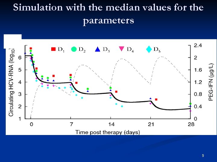Simulation with the median values for the parameters 9

Fisher Information Matrix The likelihood is given by: and hence the FIM is: By independence between the patients, the FIM for the whole sample is simply Where D is the design for the whole population D={di}i=1, …, n 10

Fisher Information Matrix n n n Cramer-Rao: the inverse of the FIM is the lower bound of the variance-covariance matrix of any unbiased estimator. The precision attainable by a design D and parameter set-up ψ is given by MF(ψ, D)-1 If parameters are estimated on their log-scale the square-root of the diagonal elements of MF(ψ, D)jj-1 are the (expected) relative errors of the parameters 11

Fisher Information Matrix n n n The likelihood has no closed-form solution The complexity of the biological model still increases the complexity of the FIM The FIM can be computed by simulations but cumbersome (not possible to optimize the FIM) By using a first order approximation around the expectation of the random effects, an analytical expression for the FIM can be obtained Here the block-diagonal matrix was used 12

The PFIM software n PFIM uses the first-order linearization and has been shown to provide very good approximation for “standard“ PK model n Recently extended to address multi-response models (www. pfim. biostat. fr) n However how does it work in such a complex ODE model ? 13

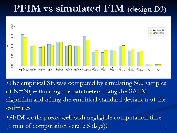PFIM vs simulated FIM (design D 3) • The empirical SE was computed by simulating 500 samples of N=30, estimating the parameters using the SAEM algorithm and taking the empirical standard deviation of the estimates • PFIM works pretty well with negligible computation time (1 min of computation versus 5 days)! 14

PFIM vs simulated FIM (design D 3) option 1 = block diagonal option 2 = full matrix

n PFIM works well in this challenging context n Designs of the literature can be compared in their ability to provide precise estimations of the parameters n Optimal designs can be found 16

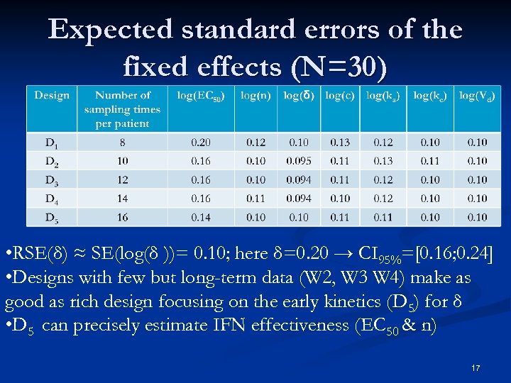Expected standard errors of the fixed effects (N=30) • RSE(δ) ≈ SE(log(δ ))= 0. 10; here δ=0. 20 → CI 95%=[0. 16; 0. 24] • Designs with few but long-term data (W 2, W 3 W 4) make as good as rich design focusing on the early kinetics (D 5) for δ • D 5 can precisely estimate IFN effectiveness (EC 50 & n) 17

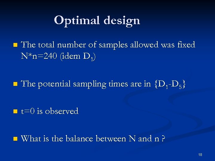Optimal design n The total number of samples allowed was fixed N*n=240 (idem D 1) n The potential sampling times are in {D 1 -D 5} n t=0 is observed n What is the balance between N and n ? 18

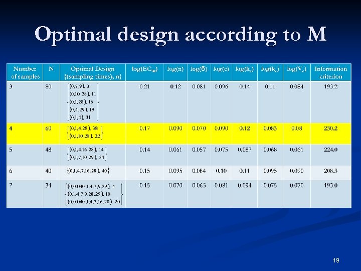Optimal design according to M 19

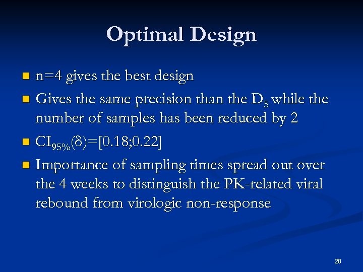Optimal Design n=4 gives the best design n Gives the same precision than the D 5 while the number of samples has been reduced by 2 n CI 95%(δ)=[0. 18; 0. 22] 95 n Importance of sampling times spread out over the 4 weeks to distinguish the PK-related viral rebound from virologic non-response n 20

Conclusion PFIM provides a very good approximation of the FIM with a negligible computation burden n The total number of sampling measurements could be reduced by half with an appropriate design n Design should not neglect long-term kinetics (W 3 & W 4) n The antiviral effectiveness of ribavirin & the kinetics of the hepatocytes cannot be estimated. n 21

Future works Predictions are done at the individual level: how to find an optimal design both at the population and at the individual level ? n To increase the number of patients is more expensive: how to include the cost in the design optimization ? n New direct-acting antivirals have a more profound effect on viral load. How to take into account the information brought by data under the level of detection ? n 22