Demand Supply Guest Lodge o o o Everyone

Demand Supply Guest Lodge o o o Everyone who handed in their assignment gets a bonus mark Groups of 4 20 minutes At the 10 minute mark can collaborate with other groups for 2 minutes Last 8 minutes you are to work in your group alone If you get 100% you will receive a second bonus mark

Chapter 5 Elasticisity of Supply and Demand

Elasticity of Demand o Would you buy the new Sony Play Station 4 if it was n n n n $2000 $1500 $1000 $800 $600 $500 $100 $20

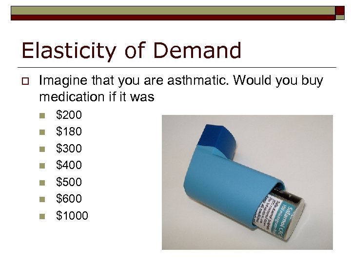Elasticity of Demand o Imagine that you are asthmatic. Would you buy medication if it was n n n n $200 $180 $300 $400 $500 $600 $1000

Elasticity of Demand o Imagine that you are NOT asthmatic. Would you buy medication if it was n n n n $1000 $800 $500 $200 $180 $5 $1

Elasticity of demand – measures how responsive demand is to price.

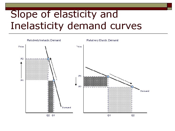
Elasticity of demand o As prices rise =>quantity demanded falls n n o o o Law of demand a change in price will lead to a large change in quantity demand (5% change in price = 10% change in demand) But by how much will sales fall? Demand for the PS 4 is elastic Demand for the asthma medication is inelastic n a change in price will lead to a small change in quantity demand (5% change in price = 2% change in demand)

Elastic Demand o When a percentage change in price causes a larger percentage change in quantity purchased n n n o i. e. A 10% increase in price causes a 50% decrease in amount purchased Buyers are price sensitive Ex Chicken Other goods that would have elastic demand?

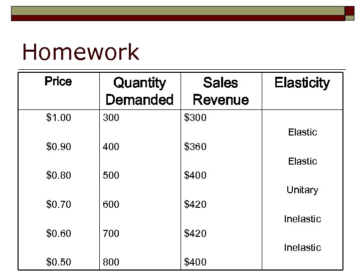
Elastic Demand & Revenue o When prices rise total revenue falls n n o Revenue = Quantity x Price Decrease in Quantity will be greater than Increase in Price When prices fall total revenue rises n n Revenue = Quantity x Price Increase in Quantity will be greater than decrease in Price

Inelastic Demand & Revenue o When prices rises total revenue rises n n o Revenue = Quantity x Price Decrease in Quantity will be smaller than Increase in Price When prices fall total revenue falls n n Revenue = Quantity x Price Increase in Quantity will be smaller than decrease in Price

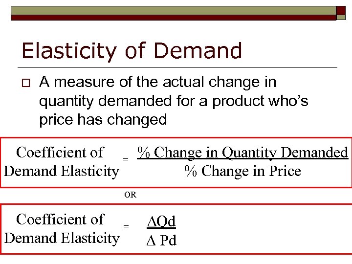Elasticity of Demand o A measure of the actual change in quantity demanded for a product who’s price has changed Coefficient of = % Change in Quantity Demanded Demand Elasticity % Change in Price OR Coefficient of = Demand Elasticity ∆Qd ∆ Pd

Elasticity of Demand o o The Cause is in the denominator The Effect is in the numerator

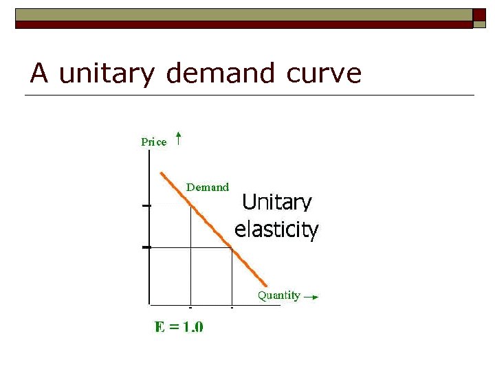
Coefficient o 1 > x : Inelastic coefficient n o 1 < x : Elastic coefficient n o Change in quantity demanded will be smaller than the change in price Change in quantity demanded will be greater than change in price 1 = x : Unitary coefficient n Change in quantity demanded will be equal to change in price (5% change in price = 5% change in demand)

Problem to solve o A large gas station sells 10 million/L of gas/month at a price of $0. 50/L. If the station’s owners raise their price to $0. 54/L the quantity demanded by the stations customers falls to 9. 5 million litres. With this information can we calculate a coefficient that the station owners will find useful in making their pricing decision?

Turn to page 95 o o Work through the equations on page 95 and 96. Fill in the table 5. 1 on page 96.

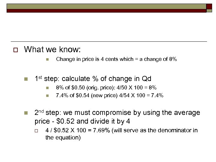o What we know: n n 1 st step: calculate % of change in Qd n n n Change in price is 4 cents which = a change of 8% 8% of $0. 50 (orig. price): 4/50 X 100 = 8% 7. 4% of $0. 54 (new price) 4/54 X 100 = 7. 4% 2 nd step: we must compromise by using the average price - $0. 52 and divide it by 4 o 4 / $0. 52 X 100 = 7. 69% (will serve as the denominator in the equation)

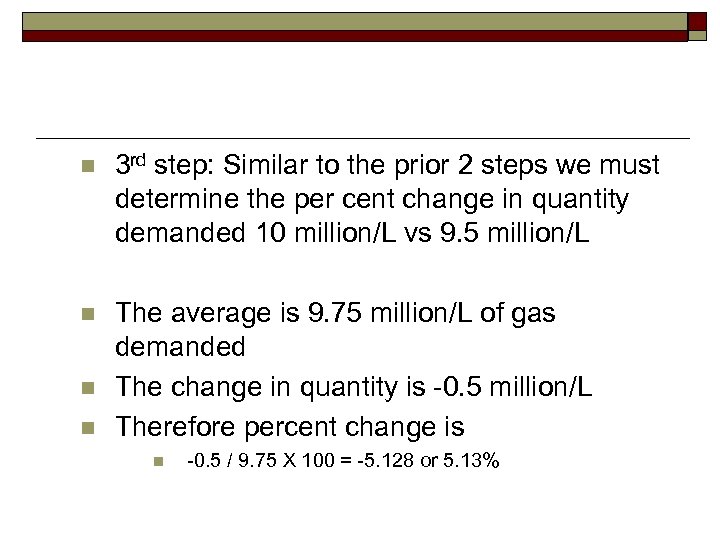n 3 rd step: Similar to the prior 2 steps we must determine the per cent change in quantity demanded 10 million/L vs 9. 5 million/L n The average is 9. 75 million/L of gas demanded The change in quantity is -0. 5 million/L Therefore percent change is n n n -0. 5 / 9. 75 X 100 = -5. 128 or 5. 13%

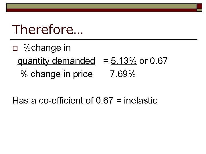Therefore… %change in quantity demanded = 5. 13% or 0. 67 % change in price 7. 69% o Has a co-efficient of 0. 67 = inelastic

Lets look at table on pg. 96

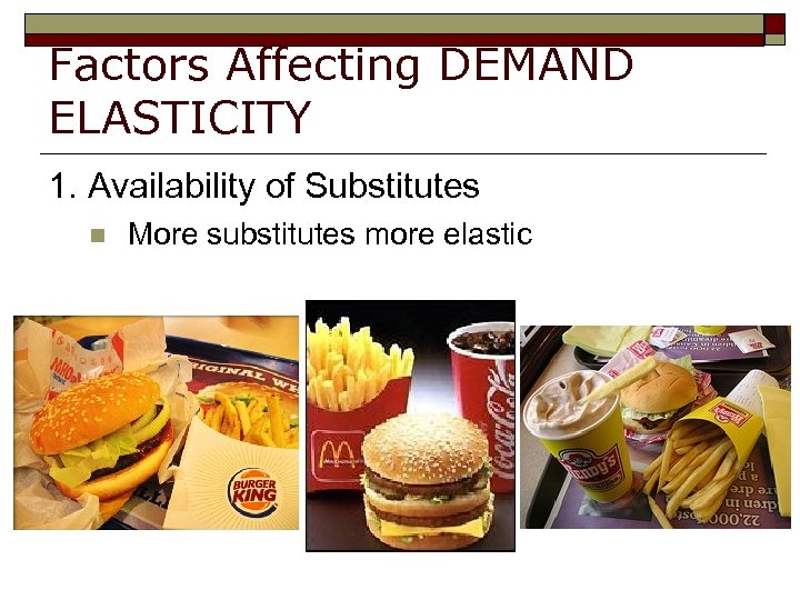Factors Affecting DEMAND ELASTICITY 1. Availability of Substitutes n More substitutes more elastic

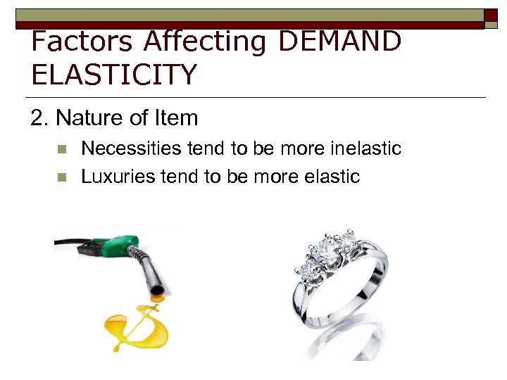Factors Affecting DEMAND ELASTICITY 2. Nature of Item n n Necessities tend to be more inelastic Luxuries tend to be more elastic

Factors Affecting DEMAND ELASTICITY 3. Fraction of income spent on item n n Big ticket item are more elastic House, Cars

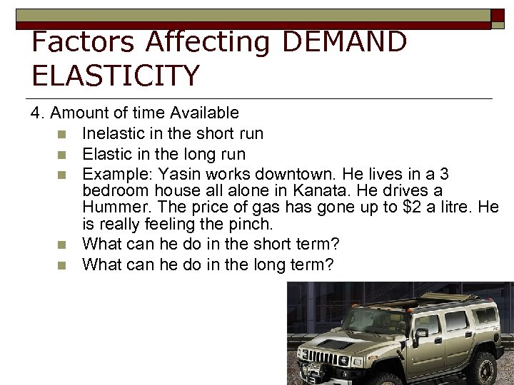Factors Affecting DEMAND ELASTICITY 4. Amount of time Available n Inelastic in the short run n Elastic in the long run n Example: Yasin works downtown. He lives in a 3 bedroom house all alone in Kanata. He drives a Hummer. The price of gas has gone up to $2 a litre. He is really feeling the pinch. n What can he do in the short term? n What can he do in the long term?

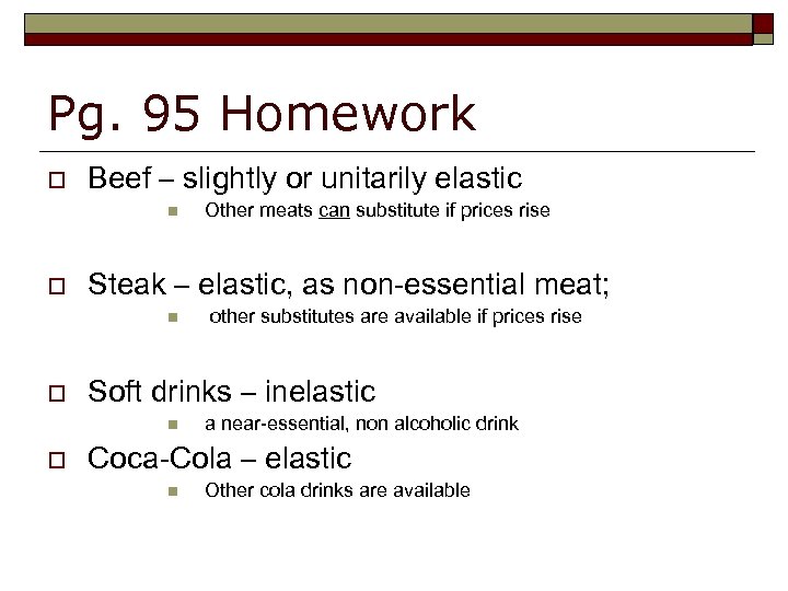Pg. 95 Homework o Beef – slightly or unitarily elastic n o Steak – elastic, as non-essential meat; n o other substitutes are available if prices rise Soft drinks – inelastic n o Other meats can substitute if prices rise a near-essential, non alcoholic drink Coca-Cola – elastic n Other cola drinks are available

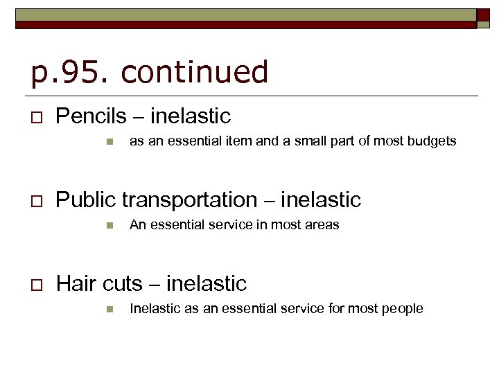p. 95. continued o Pencils – inelastic n o Public transportation – inelastic n o as an essential item and a small part of most budgets An essential service in most areas Hair cuts – inelastic n Inelastic as an essential service for most people

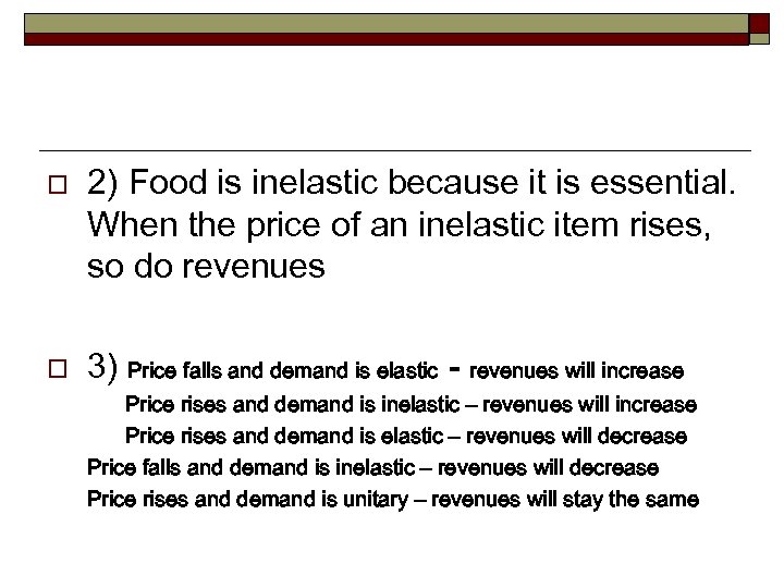o o 2) Food is inelastic because it is essential. When the price of an inelastic item rises, so do revenues 3) Price falls and demand is elastic - revenues will increase Price rises and demand is inelastic – revenues will increase Price rises and demand is elastic – revenues will decrease Price falls and demand is inelastic – revenues will decrease Price rises and demand is unitary – revenues will stay the same

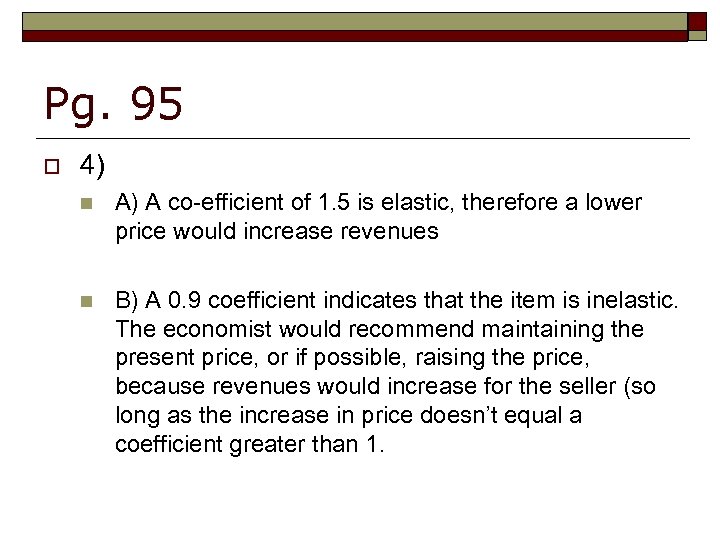Pg. 95 o 4) n A) A co-efficient of 1. 5 is elastic, therefore a lower price would increase revenues n B) A 0. 9 coefficient indicates that the item is inelastic. The economist would recommend maintaining the present price, or if possible, raising the price, because revenues would increase for the seller (so long as the increase in price doesn’t equal a coefficient greater than 1.

Slope of elasticity and Inelasticity demand curves

A unitary demand curve

Homework Price Quantity Demanded $1. 00 300 Sales Revenue Elasticity $300 Elastic $0. 90 400 $360 Elastic $0. 80 500 $400 Unitary $0. 70 600 $420 Inelastic $0. 60 700 $420 Inelastic $0. 50 800 $400

Elasticity of Supply o Elasticity of supply measures how responsive the quantity supplied by a seller is to rise or fall in price.

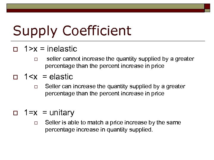Supply Coefficient o 1>x = inelastic o o 1

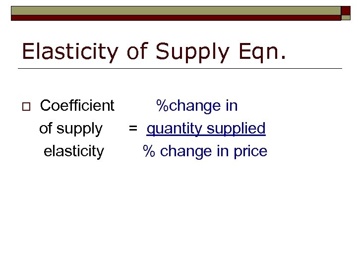Elasticity of Supply Eqn. o Coefficient %change in of supply = quantity supplied elasticity % change in price

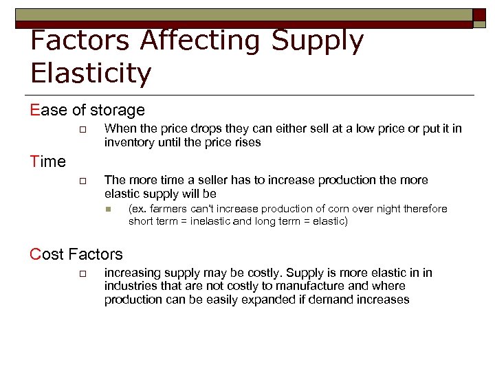Factors Affecting Supply Elasticity Ease of storage o Time o When the price drops they can either sell at a low price or put it in inventory until the price rises The more time a seller has to increase production the more elastic supply will be n Cost Factors o (ex. farmers can’t increase production of corn over night therefore short term = inelastic and long term = elastic) increasing supply may be costly. Supply is more elastic in in industries that are not costly to manufacture and where production can be easily expanded if demand increases

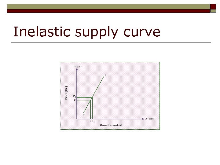Inelastic supply curve

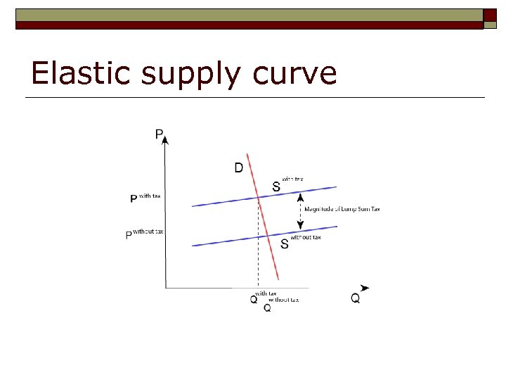Elastic supply curve

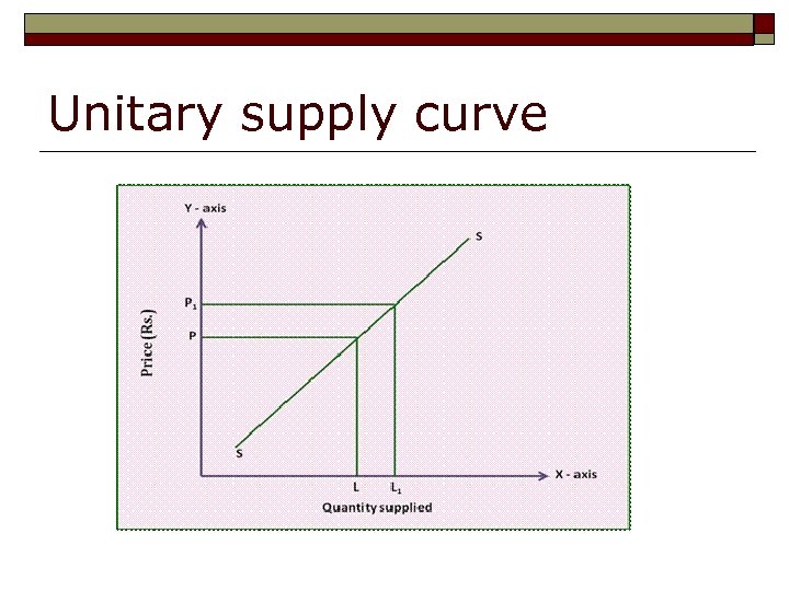Unitary supply curve

HW pg. 101 o 1) n A) A coefficient of 0. 8 is bad news for sellers, because it indicates that supply is inelastic. Thus, sellers will be slow to increase supply to take advantage of rising prices (ex. fruits and vegetables) n B) A coefficient of 1. 5 is good news for sellers because it indicates that supply is elastic. Thus sellers can quickly increase supply to take advantage or rising prices (ex. steel)

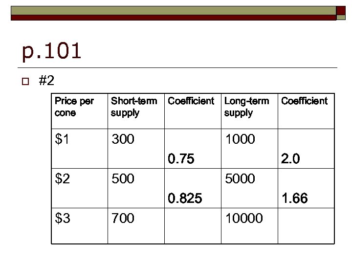p. 101 o #2 Price per cone Short-term supply $1 Coefficient 300 Long-term supply 1000 0. 75 $2 500 2. 0 5000 0. 825 $3 700 Coefficient 1. 66 10000

Utility Theory o Utility = satisfaction Marginal = extra o Marginal utility = extra satisfaction o

Example of Marginal Utility o Richard loves to eat pizza and cheeseburgers. Over the last week he has consumed 3 cheeseburgers and no pizza. While out for dinner he is looking at the menu and sees both pizza and cheeseburgers on the menu. What is he more likely to choose to eat, pizza or a cheeseburger?

o Since the marginal utility of buying a pizza will be greater than the marginal utility of buying cheeseburger, Richard will choose to buy a pizza.

o Richard is really hungry so he orders 5 o o o Consumes 1 st cheeseburger = high marginal utility Consumes 2 nd cheeseburger = marginal utility drops a bit Consumes 3 rd cheeseburger = marginal utilty drops even more By the time Richard consumes his last cheeseburger his marginal utility or extra satisfaction he gets from each additional burger is less and less. Note: n Total utility increases but less and less as each additional cheeseburger is consumed.

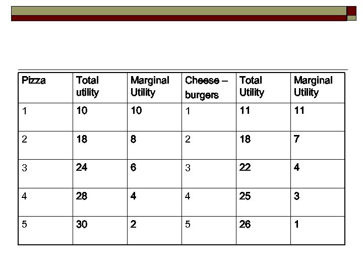Pizza Total utility Marginal Utility Cheese – burgers Total Utility Marginal Utility 1 10 10 1 11 11 2 18 8 2 18 7 3 24 6 3 22 4 4 28 4 4 25 3 5 30 2 5 26 1

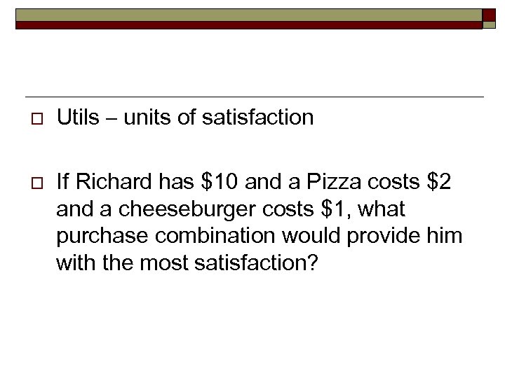o o Utils – units of satisfaction If Richard has $10 and a Pizza costs $2 and a cheeseburger costs $1, what purchase combination would provide him with the most satisfaction?

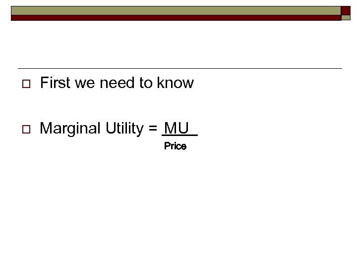o First we need to know o Marginal Utility = MU Price

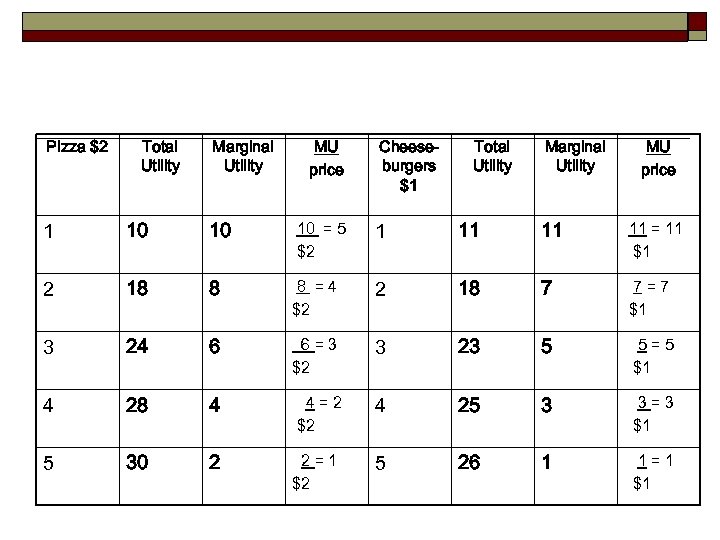Pizza $2 Total Utility Marginal Utility MU price Cheeseburgers $1 Total Utility Marginal Utility MU price 1 10 10 10 = 5 $2 1 11 11 11 = 11 $1 2 18 8 8 =4 $2 2 18 7 7=7 $1 3 24 6 6=3 $2 3 23 5 5=5 $1 4 28 4 4=2 $2 4 25 3 3=3 $1 5 30 2 2=1 $2 5 26 1 1=1 $1

o Richard’s best combination to maximize satisfaction is; o o Purchasing 3 pizzas and 4 cheeseburgers Has maximum satisfaction: 49 utils Consumer Equilibrium – receiving the same amount of satisfaction per dollar of each item Where does consumer equilibrium occur for Richard?

Pg. 105 HW o 1) The total satisfaction from consumeing several soft drinks is higher than consuming just one, but the extra satisfaction gained from each drink after the first one drops steadily

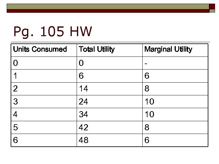Pg. 105 HW Units Consumed Total Utility Marginal Utility 0 0 - 1 6 6 2 14 8 3 24 10 4 34 10 5 42 8 6 48 6

o 3) Enrique’s consumer surplus is $2 because he would have paid $10 for one movie, but now he has to pay only $8.

Consumer Surplus o o Consumer surplus – the difference between what consumers are wiling to pay for an item and what they actually pay Ex. o IPAD 3 is $800 but you would have paid $1000 = consumer surplus of $200

Ceiling Price o o o A price restriction place by government in order to prevent the price of a product from rising above a certain level Results in a shortage if the ceiling price is lower than the equilibrium price Ex Gas Prices, Rent Control

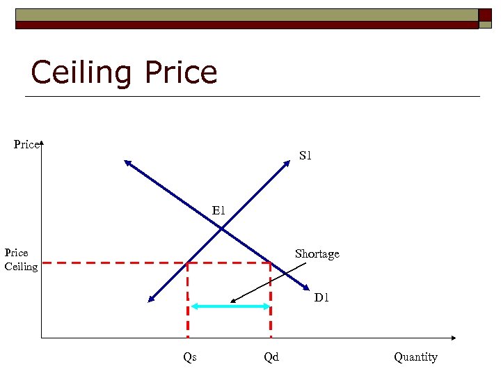Ceiling Price S 1 E 1 Price Ceiling Shortage D 1 Qs Qd Quantity

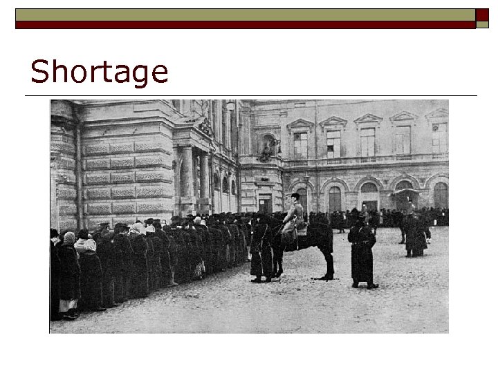Shortage

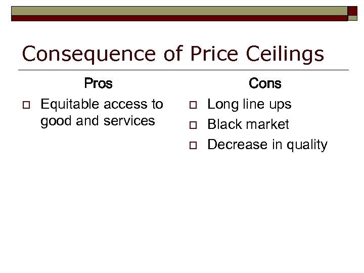Consequence of Price Ceilings o Pros Equitable access to good and services o o o Cons Long line ups Black market Decrease in quality

Floor Price o o o A price restriction placed by government in order to prevent the price of a product from falling below a certain level Results in a surplus if the price is above the equilibrium price Ex Minimum Wage

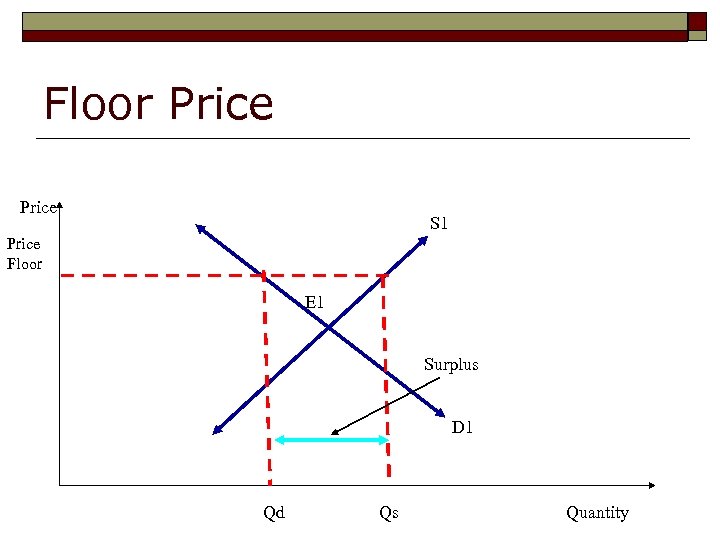Floor Price S 1 Price Floor E 1 Surplus D 1 Qd Qs Quantity

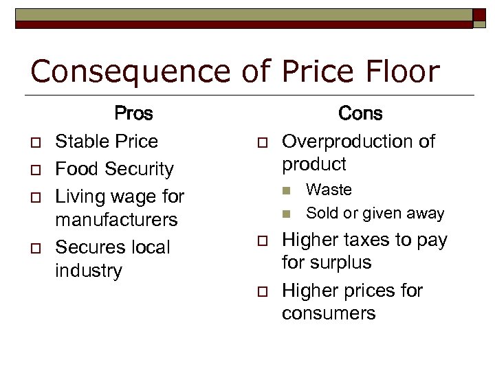Consequence of Price Floor o o Pros Stable Price Food Security Living wage for manufacturers Secures local industry o Cons Overproduction of product n n o o Waste Sold or given away Higher taxes to pay for surplus Higher prices for consumers

Subsidies o o o A grant of money made to particular industry by the government Results in a supply shift to the right Example n n n Farm Subsidies Research and Development New Industry (Infant Industry) o Environmental

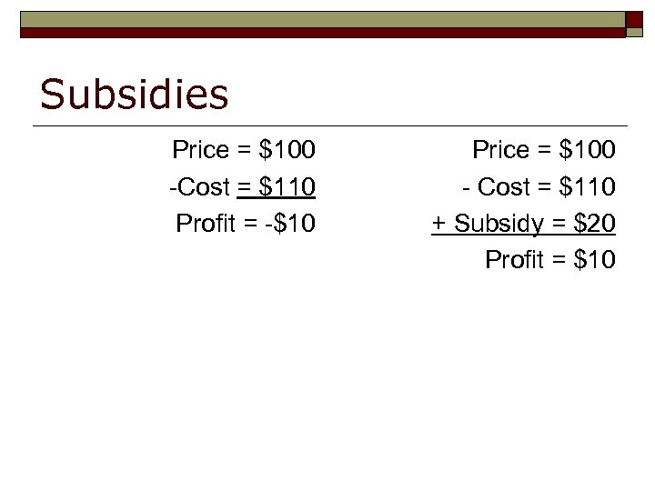Subsidies Price = $100 -Cost = $110 Profit = -$10 Price = $100 - Cost = $110 + Subsidy = $20 Profit = $10

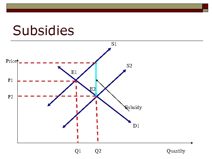Subsidies S 1 Price S 2 E 1 P 1 E 2 P 2 Subsidy D 1 Q 2 Quantity

Subsidies

o o http: //www. cbsnews. com/video/watch/? id =3516785 n http: //vimeo. com/6184633