Demand Supply and Elasticity Applications and Exercises Lecture

Demand, Supply and Elasticity: Applications and Exercises Lecture 3 – academic year 2014/15 Introduction to Economics Fabio Landini

Ex. 3. 1 – The lottery Question Suppose you win 100 € at the lottery. You can spend all the money in beers or invest them at 5%. How much does it cost to spend the money you win in beers? Hint: Reason in terms of opportunity cost…

Ex. 3. 1 – The lottery Answer By investing 100 € today you would obtain 105 € tomorrow. Therefore: the opportunity cost of beer is 105 €, that is the amount of money you renounce to buy beers.

Ex. 3. 2 – Product development Question A company invested 5 mln. € to develop a new product, expecting an equal return from the investment. Problem: 5 mln are not enough to complete the product, 1 mln more is needed. Moreover: competition reduces the expectation to just 3 mln € sales. Is it more convenient to stop or to continue the commercialization of the product? Hint: Reason in terms of MB vs. MC

Ex. 3. 3 – Product development Answer It is convenient to continue, because MC < MB MC = 1 mln € MB = 3 mln € In this way you can contain losses… If the company stops: costs = 5 mln €, revenues = 0 mln € => losses = 5 mln € If the company continues: costs = 6 mln €, revenues = 3 mln € => losses = 3 mln €

Ex. 3. 3 – Demand Supply I Question Use the Demand & Supply model to answer the following questions: i) When a chill hits Sicily, what happens to the price of oranges in Italy? Increases or decrease? ii) When UK benefits of a mild winter, what happens to the price of hotel rooms in Costa Brava? Increase or decrease? iii) When a war breaks out in Middle East, what happens to the price of petrol an second-hand Cadillac in US? Increase or decrease?

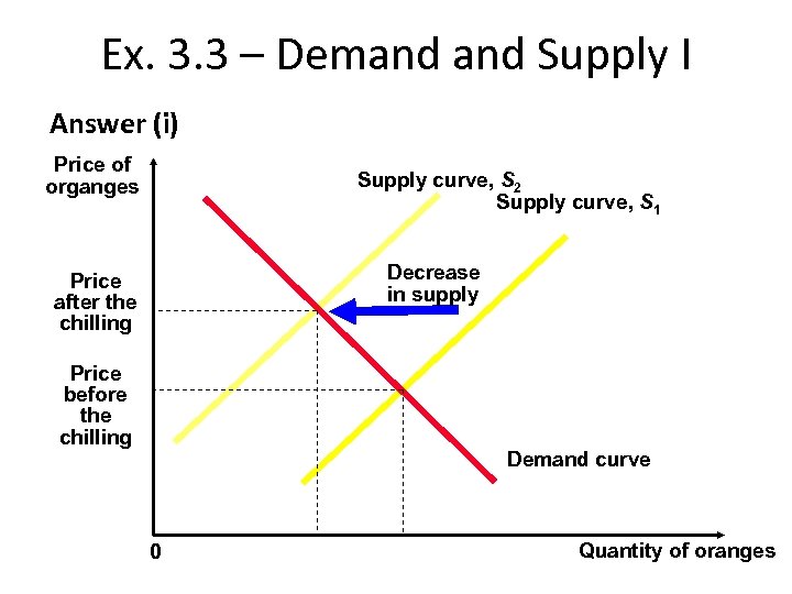Ex. 3. 3 – Demand Supply I Answer (i) Price of organges Supply curve, S 2 Supply curve, S 1 Decrease in supply Price after the chilling Price before the chilling Demand curve 0 Quantity of oranges

Ex. 3. 3 – Demand Supply I Answer (ii) In this case mild winter in UK and hotel rooms in Costa Brava are SUBSTITUTE goods. The nice weather reduces the UK’s demand for holidays abroad, and thus it diminishes the demand on the market for hotel rooms in Costa Brava.

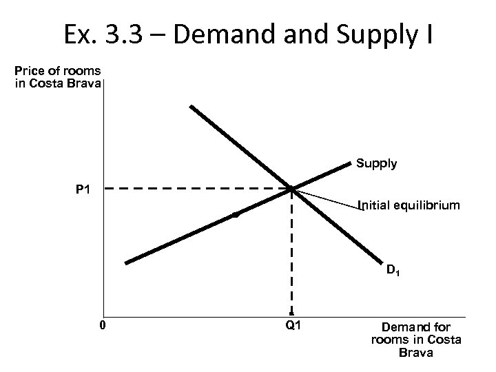Ex. 3. 3 – Demand Supply I Price of rooms in Costa Brava Supply P 1 Initial equilibrium D 1 0 Q 1 Demand for rooms in Costa Brava

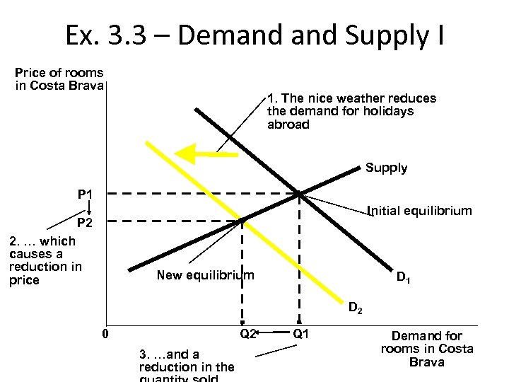Ex. 3. 3 – Demand Supply I Price of rooms in Costa Brava 1. The nice weather reduces the demand for holidays abroad Supply P 1 Initial equilibrium P 2 2. … which causes a reduction in price New equilibrium D 1 D 2 0 Q 2 3. …and a reduction in the Q 1 Demand for rooms in Costa Brava

Ex. 3. 3 – Demand Supply I Answer (iii) The price of petrol increases, because the supply of oil from the countries that take part to the conflict reduces. The value of second-hand Cadillac reduces remarkably, because they consume a lot of petrol. All wants to buy cars that consumes less petrol. Cadillac and petrol are COMPLEMENYTARY goods.

Ex. 3. 4 – Demand Supply II Question The market for cheese is characterized by the following demand supply curve: Demand: QD= 9 – P Supply: QO= 3 P – 3 where P represent the price (in Euro per Kg. ) and Q represent the quantity (in Kg. ). How do the demand curve and supply curve look like (draw)? Which is the value of the equilibrium prices and quantities?

Ex. 3. 4 – Demand Supply II Solution: Both the demand supply curves are straight lines of the type y = a + bx , where y=Q and x=P. For instance, in our case: – for the demand: a = 9 and b= – 1 – for the supply: a = – 3 and b= 3 Important: Usually, the two curves are drawn with P on the vertical axis and Q on the horizontal axis.

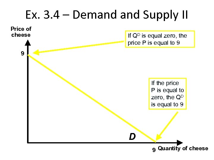Ex. 3. 4 – Demand Supply II Price of cheese If QD is equal zero, the price P is equal to 9 9 If the price P is equal to zero, the QD is equal to 9 D 9 Quantity of cheese

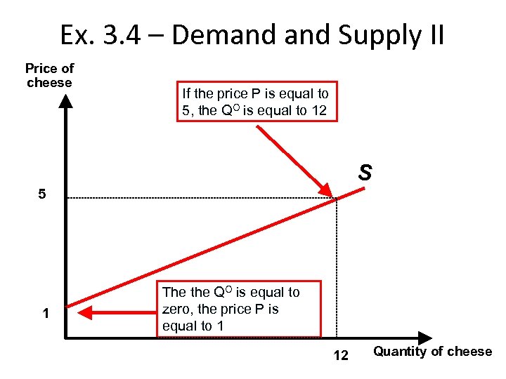Ex. 3. 4 – Demand Supply II Price of cheese If the price P is equal to 5, the QO is equal to 12 S 5 1 The the QO is equal to zero, the price P is equal to 1 12 Quantity of cheese

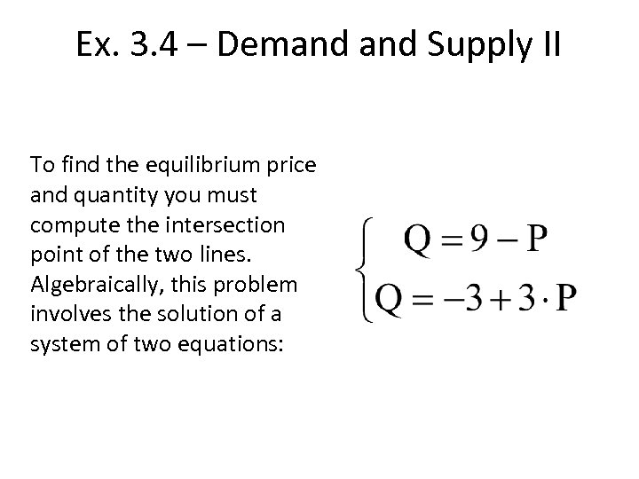Ex. 3. 4 – Demand Supply II To find the equilibrium price and quantity you must compute the intersection point of the two lines. Algebraically, this problem involves the solution of a system of two equations:

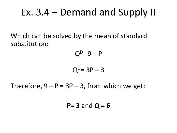Ex. 3. 4 – Demand Supply II Which can be solved by the mean of standard substitution: QD = 9 – P QO= 3 P – 3 Therefore, 9 – P = 3 P – 3, from which we get: P= 3 and Q = 6

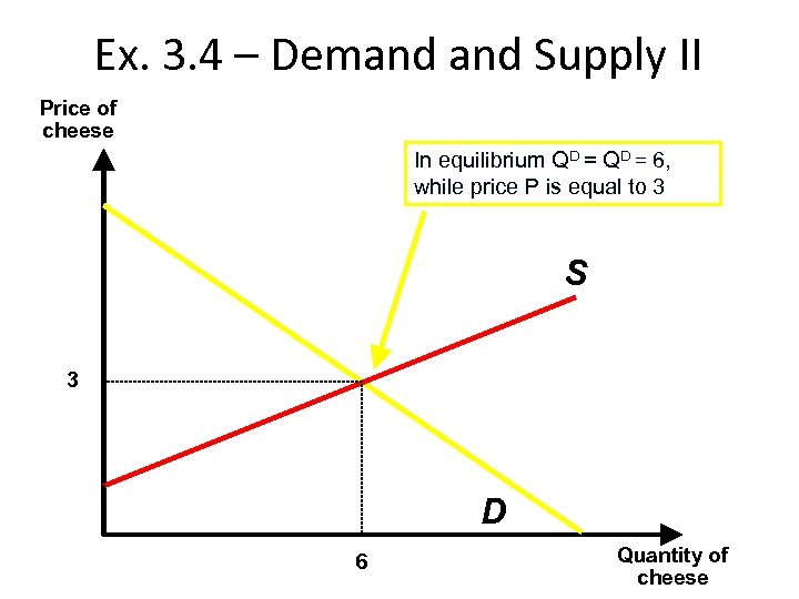Ex. 3. 4 – Demand Supply II Price of cheese In equilibrium QD = 6, while price P is equal to 3 S 3 D 6 Quantity of cheese

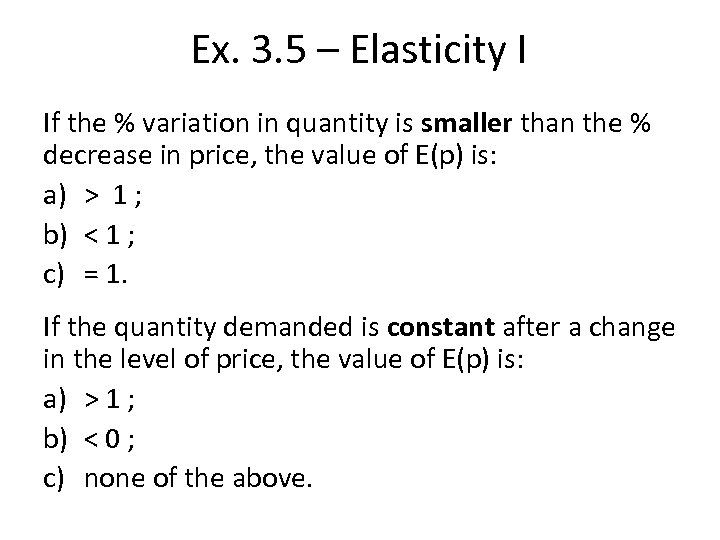Ex. 3. 5 – Elasticity I If the % variation in quantity is smaller than the % decrease in price, the value of E(p) is: a) > 1 ; b) < 1 ; c) = 1. If the quantity demanded is constant after a change in the level of price, the value of E(p) is: a) > 1 ; b) < 0 ; c) none of the above.

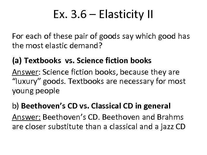Ex. 3. 6 – Elasticity II For each of these pair of goods say which good has the most elastic demand? (a) Textbooks vs. Science fiction books Answer: Science fiction books, because they are “luxury” goods. Textbooks are necessary for most young people b) Beethoven’s CD vs. Classical CD in general Answer: Beethoven’s CD. Beethoven and Brahms are closer substitute than a classical and a jazz CD

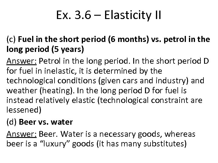Ex. 3. 6 – Elasticity II (c) Fuel in the short period (6 months) vs. petrol in the long period (5 years) Answer: Petrol in the long period. In the short period D for fuel in inelastic, it is determined by the technological conditions (given cars and industry) and weather (heating). In the long period D for fuel is instead relatively elastic (technological constraint are lessened) (d) Beer vs. water Answer: Beer. Water is a necessary goods, whereas beer is a “luxury” goods (it has many substitutes)

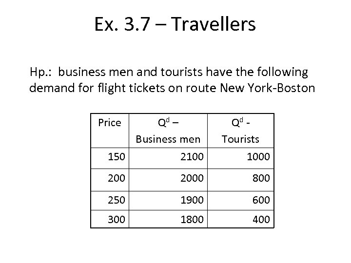Ex. 3. 7 – Travellers Hp. : business men and tourists have the following demand for flight tickets on route New York-Boston Price Qd – Business men 150 2100 Qd Tourists 1000 2000 800 250 1900 600 300 1800 400

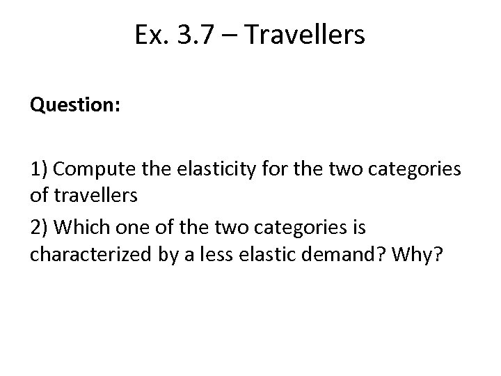Ex. 3. 7 – Travellers Question: 1) Compute the elasticity for the two categories of travellers 2) Which one of the two categories is characterized by a less elastic demand? Why?

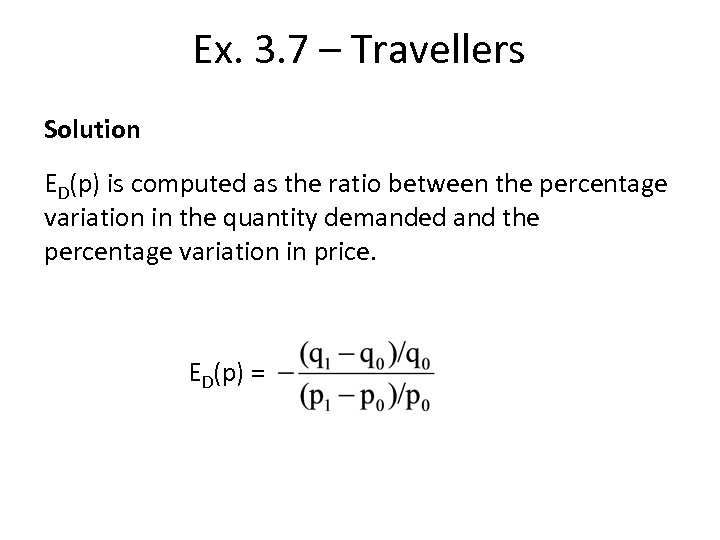Ex. 3. 7 – Travellers Solution ED(p) is computed as the ratio between the percentage variation in the quantity demanded and the percentage variation in price. ED(p) =

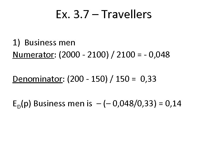Ex. 3. 7 – Travellers 1) Business men Numerator: (2000 - 2100) / 2100 = - 0, 048 Denominator: (200 - 150) / 150 = 0, 33 ED(p) Business men is – (– 0, 048/0, 33) = 0, 14

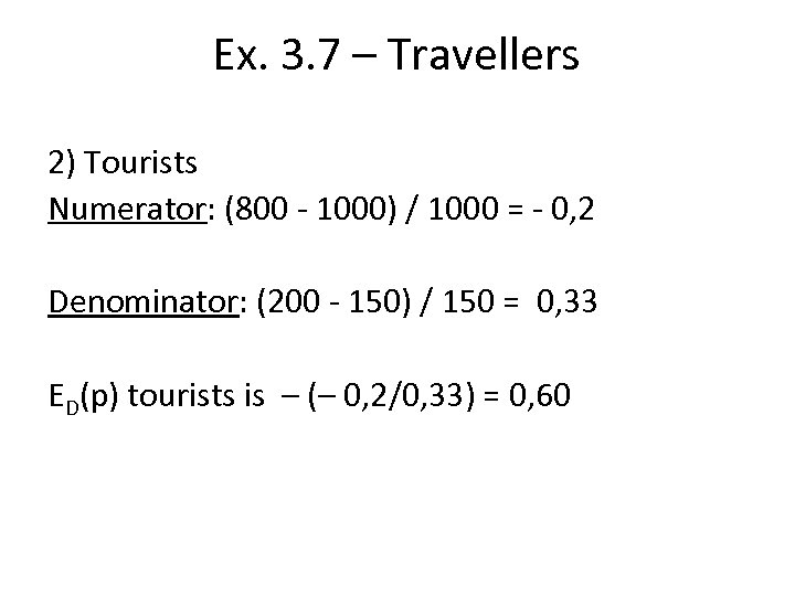Ex. 3. 7 – Travellers 2) Tourists Numerator: (800 - 1000) / 1000 = - 0, 2 Denominator: (200 - 150) / 150 = 0, 33 ED(p) tourists is – (– 0, 2/0, 33) = 0, 60

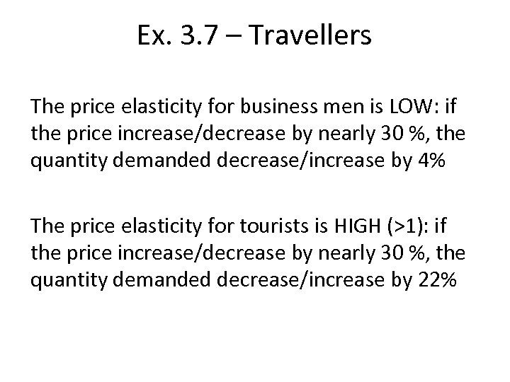Ex. 3. 7 – Travellers The price elasticity for business men is LOW: if the price increase/decrease by nearly 30 %, the quantity demanded decrease/increase by 4% The price elasticity for tourists is HIGH (>1): if the price increase/decrease by nearly 30 %, the quantity demanded decrease/increase by 22%

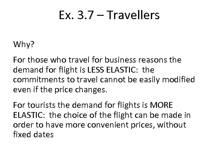Ex. 3. 7 – Travellers Why? For those who travel for business reasons the demand for flight is LESS ELASTIC: the commitments to travel cannot be easily modified even if the price changes. For tourists the demand for flights is MORE ELASTIC: the choice of the flight can be made in order to have more convenient prices, without fixed dates

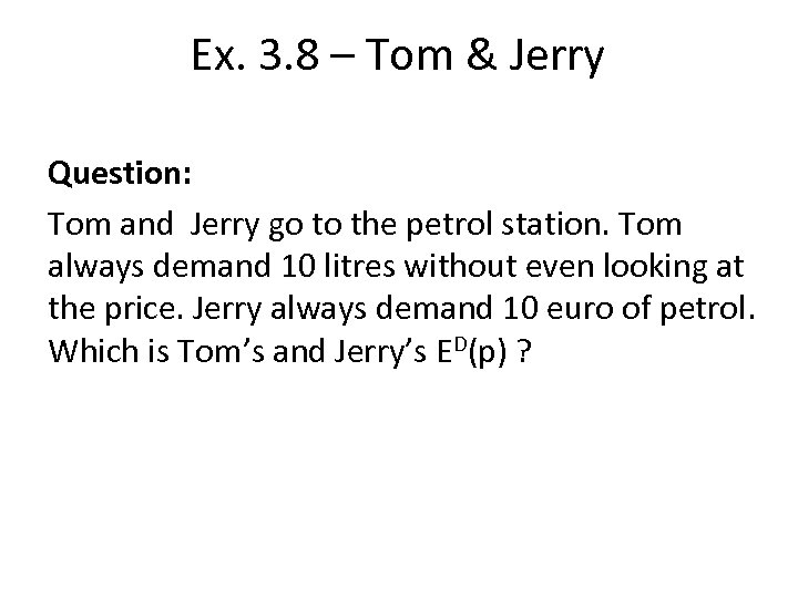Ex. 3. 8 – Tom & Jerry Question: Tom and Jerry go to the petrol station. Tom always demand 10 litres without even looking at the price. Jerry always demand 10 euro of petrol. Which is Tom’s and Jerry’s ED(p) ?

Ex. 3. 8 – Tom & Jerry Answer: Tom’s ED(p) is equal zero, since he wants the same quantity regardless of the price. Jerry’s ED(p) is 1, since he spends the same amount on gas, no matter what the price, which means his percentage change in quantity is equal to the percentage change in price.