Demand Estimation Chapter 5 2009 2006 South-Western

Demand Estimation Chapter 5 © 2009, 2006 South-Western, a part of Cengage Learning

Chapter 5 OVERVIEW Ø Ø Ø Ø Interview and Experimental Methods Simple Demand Curve Estimation Simple Market Demand Curve Estimation Identification Problem Regression Analysis Measuring Regression Model Significance Measures of Individual Variable Significance © 2009, 2006 South-Western, a part of Cengage Learning

Chapter 5 KEY CONCEPTS Ø Ø Ø market demand curve simultaneous relation identification problem consumer interview market experiments regression analysis deterministic relation statistical relation time series cross section scatter diagram linear model Ø Ø Ø multiplicative model simple regression model multiple regression model standard error of the estimate (SEE) correlation coefficient of determination degrees of freedom corrected coefficient of determination F statistic two-tail t tests one‑tail t tests © 2009, 2006 South-Western, a part of Cengage Learning

Interview and Experimental Methods Ø Consumer Interviews l l Interviews can solicit useful information when market data is scarce. Consumer opinions can differ from behavior. Ø Market Experiments l l Controlled experiments can generate useful insight. Experiments can be expensive. © 2009, 2006 South-Western, a part of Cengage Learning

Another possibility is for the firm to introduce new products, or increase quality or an existing product. The firm can analyze the change in demand. All firms experiment in one way or another. They run advertising campaigns and monitor sales, they increase/decrease prices and monitor sales. © 2009, 2006 South-Western, a part of Cengage Learning

Simple Demand Curve Estimation Ø Simple Linear Demand Curves l l The best estimation method balances marginal costs and marginal benefits. Simple linear relations are often useful for demand estimation. Ø Using Simple Linear Demand Curves l Straight-line relations can give useful approximations. © 2009, 2006 South-Western, a part of Cengage Learning

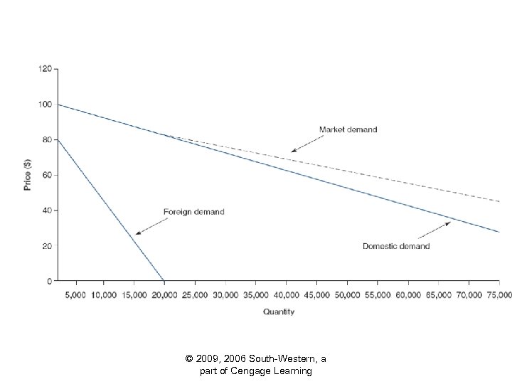
Simple Market Demand Curve Estimation Ø Market Demand Curve l Shows total quantity customers are willing to buy at various prices under current market conditions. Ø Graphing the Market Demand Curve l l Market demand is the sum of individual demand quantities, Q 1 + Q 2 = Q 1+2. Add quantities, not prices! © 2009, 2006 South-Western, a part of Cengage Learning

© 2009, 2006 South-Western, a part of Cengage Learning

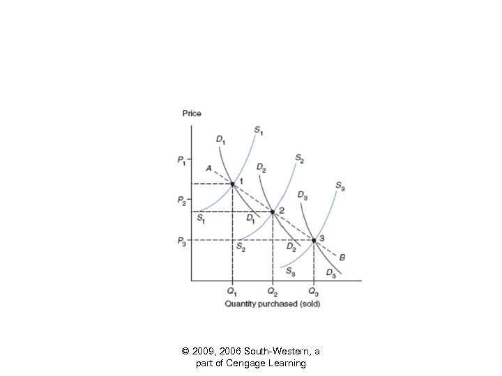
Identification Problem Ø Changing Nature of Demand Relations l Demand relations are dynamic. Ø Interplay of Demand Supply l Economic conditions affect demand supply. Ø Shifts in Demand Supply l Curve shifts can be estimated. Ø Simultaneous Relations l Quantity and price are jointly determined. © 2009, 2006 South-Western, a part of Cengage Learning

© 2009, 2006 South-Western, a part of Cengage Learning

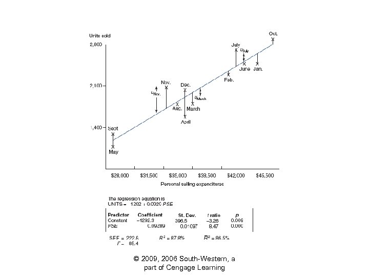
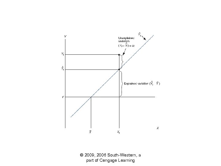
Regression Analysis Ø What Is a Statistical Relation? l l A statistical relation exists when averages are related. A deterministic relation is true by definition. Ø Specifying the Regression Model l l Dependent variable Y is caused by X. X variables are independently determined from Y. Ø Least Squares Method l © 2009, 2006 South-Western, a part of Cengage Learning Minimize sum of squared residuals.

© 2009, 2006 South-Western, a part of Cengage Learning

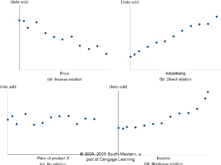
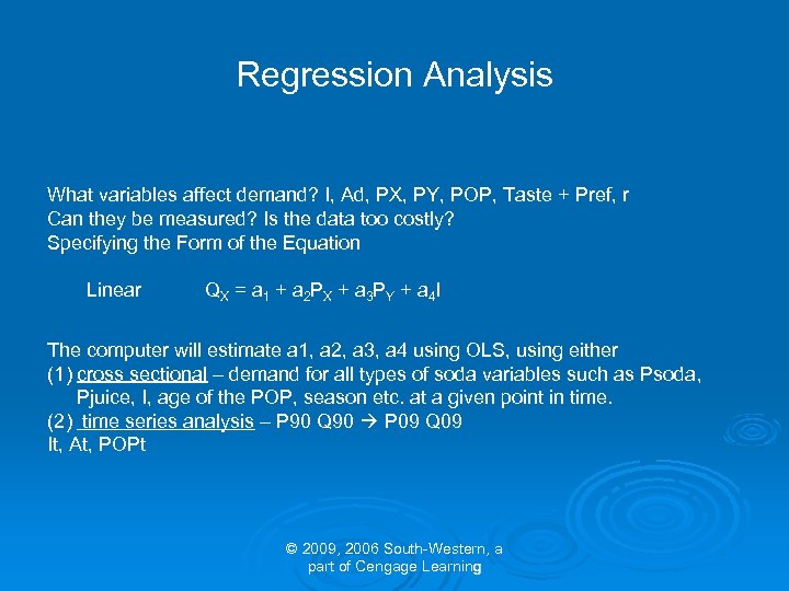Regression Analysis What variables affect demand? I, Ad, PX, PY, POP, Taste + Pref, r Can they be measured? Is the data too costly? Specifying the Form of the Equation Linear QX = a 1 + a 2 PX + a 3 PY + a 4 I The computer will estimate a 1, a 2, a 3, a 4 using OLS, using either (1) cross sectional – demand for all types of soda variables such as Psoda, Pjuice, I, age of the POP, season etc. at a given point in time. (2) time series analysis – P 90 Q 90 P 09 Q 09 It, At, POPt © 2009, 2006 South-Western, a part of Cengage Learning

© 2009, 2006 South-Western, a part of Cengage Learning

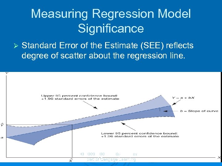Measuring Regression Model Significance Ø Standard Error of the Estimate (SEE) reflects degree of scatter about the regression line. © 2009, 2006 South-Western, a part of Cengage Learning

© 2009, 2006 South-Western, a part of Cengage Learning

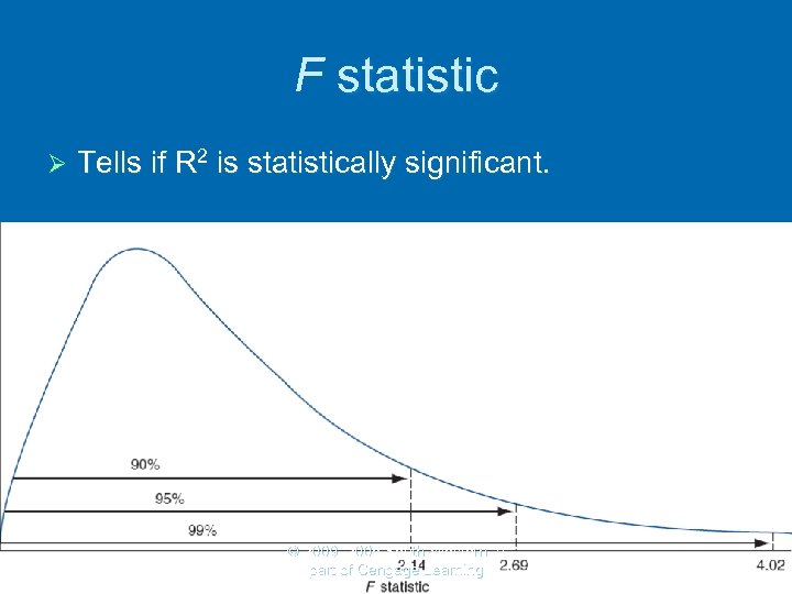F statistic Ø Tells if R 2 is statistically significant. © 2009, 2006 South-Western, a part of Cengage Learning

Goodness of Fit Ø Correlation shows degree of concurrence. l l r = 1 means perfect correlation. r = 0 means no correlation. Ø Coefficient of determination, R 2. l l R 2 = 100% means perfect fit. R 2 = 0% means no relation. Ø Corrected coefficient of determination l Adjusts R 2 downward for small samples. © 2009, 2006 South-Western, a part of Cengage Learning

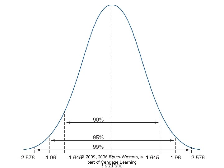
Judging Variable Significance Ø t statistics compare sample characteristics to the standard deviation of that characteristic. l l Ø Two-tail t Tests l Ø t > 2 implies a strong effect of X on Y (95% conf. ). t > 3 implies a very strong effect of X on Y (99% conf. ) Tests of effect. One-Tail t Tests l Tests of magnitude or direction. © 2009, 2006 South-Western, a part of Cengage Learning

Multiplicative Model QX = APXB PYC IR AE POPF The marginal effect on demand of any of the independent variables depends on the value (levels) of the other variables. Proof is in the book. A Company’s advertising may be more effective when I is high. But more importantly the exponents are equal to the elasticity of each variable. Proof (d. Qx/d. I) (I/Qx) = e. I (d. Qx/d. I) (I/Qx) = APXB PYC IR AE POPF Notice no matter what the value is of QXI the elasticity = d; this is called constant elasticity of demand. Log Q = Log A + B Log PX + C Log PY + D Log I + C Log A + F Log POP Computer Packages Transform Data Into Logs Elasticity varies using the linear form… Which one is better? It depends on the data. © 2009, 2006 South-Western, a part of Cengage Learning

Case Study Ø Mrs. Smyth’s Gourmet Pies Ø Page 195 © 2009, 2006 South-Western, a part of Cengage Learning

© 2009, 2006 South-Western, a part of Cengage Learning