Demand Analysis Chapter 3 Demand Relationships

Demand Analysis Chapter 3 • Demand Relationships • The Price Elasticity of Demand » Arc and point price elasticity » Elasticity and revenue relationships » Why some products are inelastic and others are elastic • Income Elasticities • Cross Elasticities of Demand • Combined Effects of Elasticities © 2011 Cengage Learning. All Rights Reserved. May not be scanned, copied or duplicated, or posted to a publicly accessible website, in whole or in part. Slide 1

Health Care & Cigarettes • Raising cigarette taxes reduces smoking » In Canada, over $4 for a pack of cigarettes reduced smoking 38% in a decade • But cigarette taxes also helps fund health care initiatives » The issue then, should we find a tax rate that maximizes tax revenues? » Or a tax rate that reduces smoking? Slide 2

Demand Analysis • An important contributor to firm risk arises from sudden shifts in demand for the product or service. • Demand analysis serves two managerial objectives: (1) it provides the insights necessary for effective management of demand, and (2) it aids in forecasting sales and revenues. Slide 3

Downward Slope to the Demand Curve • Economists presume consumers are maximizing their utility • This is used to derive a demand curve from utility maximization » income effect -- as the price of a good declines, the consumer can purchase more of all goods since his or her real income increased. So as the price falls, we typically buy more. » substitution effect -- as the price declines, the good becomes relatively cheaper. A rational consumer maximizes satisfaction by reorganizing consumption until the marginal utility in each good per dollar is equal. We buy more. » targeting, switching, and positioning – marketing efforts such as loyalty programs affect demand. Slide 4

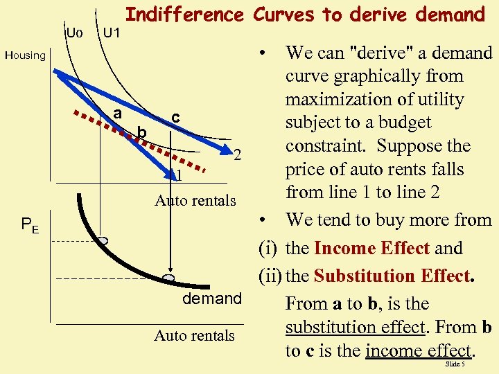Uo Housing PE U 1 Indifference Curves to derive demand • We can "derive" a demand curve graphically from maximization of utility a c subject to a budget b constraint. Suppose the 2 price of auto rents falls 1 from line 1 to line 2 Auto rentals • We tend to buy more from (i) the Income Effect and (ii) the Substitution Effect. demand From a to b, is the substitution effect. From b Auto rentals to c is the income effect. Slide 5

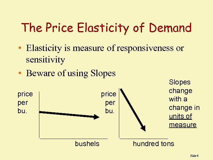The Price Elasticity of Demand • Elasticity is measure of responsiveness or sensitivity • Beware of using Slopes price per bu. bushels Slopes change with a change in units of measure hundred tons Slide 6

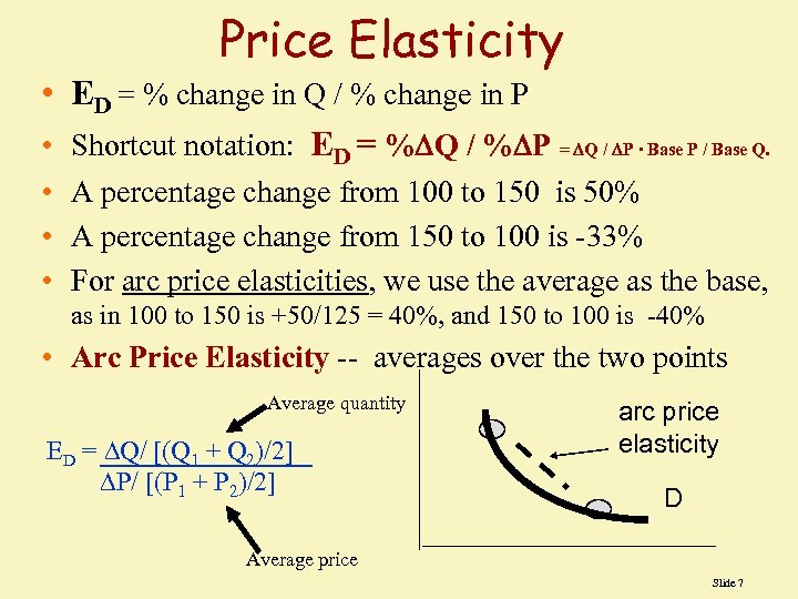Price Elasticity • ED = % change in Q / % change in P • Shortcut notation: ED = % Q / % P = Q / P ∙ Base P / Base Q. • A percentage change from 100 to 150 is 50% • A percentage change from 150 to 100 is -33% • For arc price elasticities, we use the average as the base, as in 100 to 150 is +50/125 = 40%, and 150 to 100 is -40% • Arc Price Elasticity -- averages over the two points Average quantity ED = Q/ [(Q 1 + Q 2)/2] P/ [(P 1 + P 2)/2] arc price elasticity D Average price Slide 7

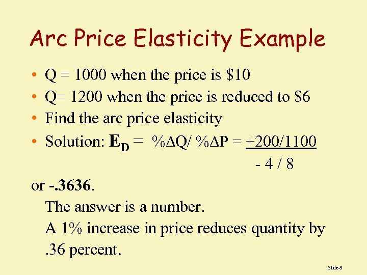Arc Price Elasticity Example • • Q = 1000 when the price is $10 Q= 1200 when the price is reduced to $6 Find the arc price elasticity Solution: ED = % Q/ % P = +200/1100 -4/8 or -. 3636. The answer is a number. A 1% increase in price reduces quantity by. 36 percent. Slide 8

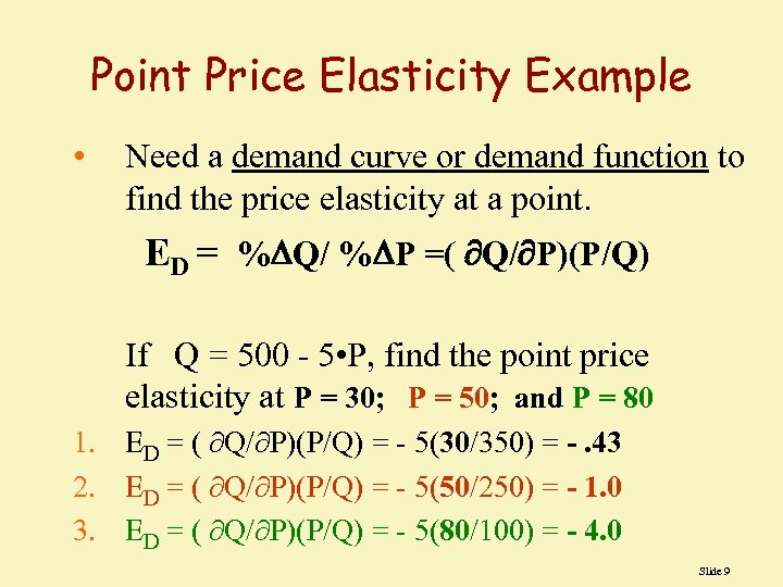Point Price Elasticity Example • Need a demand curve or demand function to find the price elasticity at a point. ED = % Q/ % P =( Q/ P)(P/Q) If Q = 500 - 5 • P, find the point price elasticity at P = 30; P = 50; and P = 80 1. ED = ( Q/ P)(P/Q) = - 5(30/350) = -. 43 2. ED = ( Q/ P)(P/Q) = - 5(50/250) = - 1. 0 3. ED = ( Q/ P)(P/Q) = - 5(80/100) = - 4. 0 Slide 9

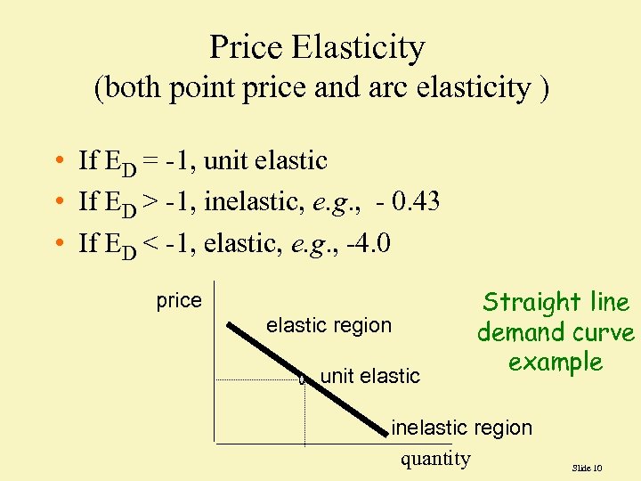Price Elasticity (both point price and arc elasticity ) • If ED = -1, unit elastic • If ED > -1, inelastic, e. g. , - 0. 43 • If ED < -1, elastic, e. g. , -4. 0 price elastic region unit elastic Straight line demand curve example inelastic region quantity Slide 10

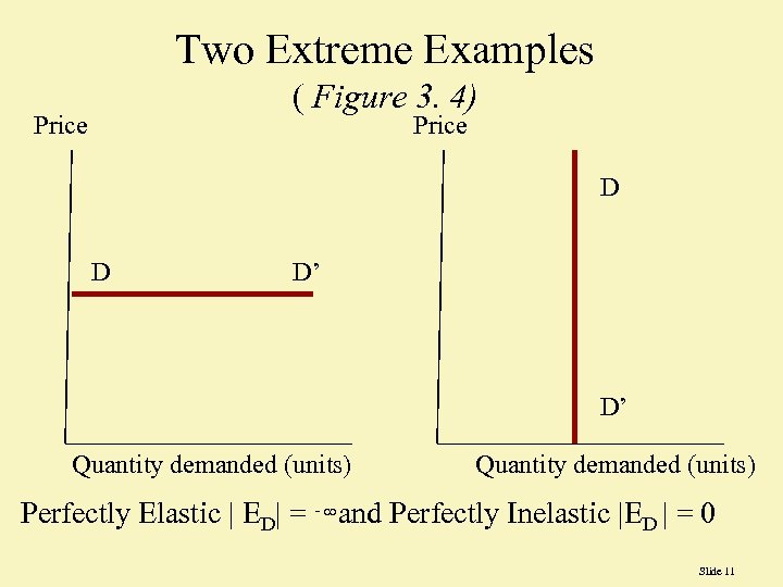Two Extreme Examples ( Figure 3. 4) Price D D D’ D’ Quantity demanded (units) and Perfectly Inelastic |E | = 0 Perfectly Elastic | ED| = D - Slide 11

TR and Price Elasticities • If you raise price, does TR rise? • Suppose demand is elastic, and raise price. TR = P • Q, so, % TR = % P+ % Q • If elastic, P , but Q a lot • Hence TR FALLS !!! • Suppose demand is inelastic, and we decide to raise price. What happens to TR and TC and profit? Slide 12

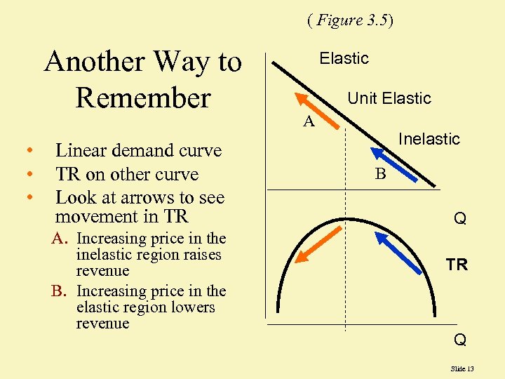( Figure 3. 5) Another Way to Remember • • • Linear demand curve TR on other curve Look at arrows to see movement in TR A. Increasing price in the inelastic region raises revenue B. Increasing price in the elastic region lowers revenue Elastic Unit Elastic A Inelastic B Q TR Q Slide 13

MR and Elasticity • Marginal revenue is TR / Q • To sell more, often price must decline, so MR is often less than the price. à MR = P ( 1 + 1/ED ) equation 3. 7 • For a perfectly elastic demand, ED = -B. Hence, MR = P. • If ED = -2, then MR =. 5 • P, or is half of the price. Slide 14

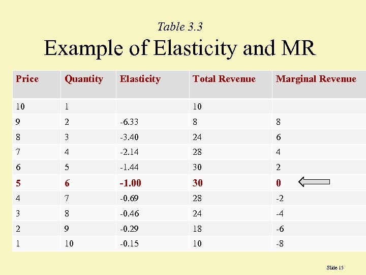Table 3. 3 Example of Elasticity and MR Price Quantity Elasticity Total Revenue Marginal Revenue 10 1 9 2 -6. 33 8 8 8 3 -3. 40 24 6 7 4 -2. 14 28 4 6 5 -1. 44 30 2 5 6 -1. 00 30 0 4 7 -0. 69 28 -2 3 8 -0. 46 24 -4 2 9 -0. 29 18 -6 1 10 -0. 15 10 -8 10 Slide 15

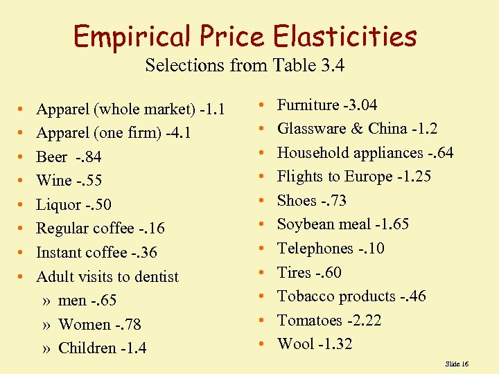Empirical Price Elasticities Selections from Table 3. 4 • • Apparel (whole market) -1. 1 Apparel (one firm) -4. 1 Beer -. 84 Wine -. 55 Liquor -. 50 Regular coffee -. 16 Instant coffee -. 36 Adult visits to dentist » men -. 65 » Women -. 78 » Children -1. 4 • • • Furniture -3. 04 Glassware & China -1. 2 Household appliances -. 64 Flights to Europe -1. 25 Shoes -. 73 Soybean meal -1. 65 Telephones -. 10 Tires -. 60 Tobacco products -. 46 Tomatoes -2. 22 Wool -1. 32 Slide 16

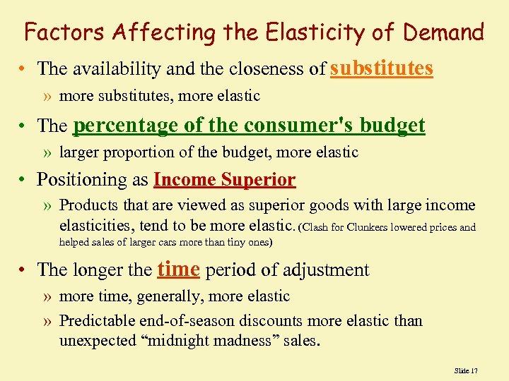Factors Affecting the Elasticity of Demand • The availability and the closeness of substitutes » more substitutes, more elastic • The percentage of the consumer's budget » larger proportion of the budget, more elastic • Positioning as Income Superior » Products that are viewed as superior goods with large income elasticities, tend to be more elastic. (Clash for Clunkers lowered prices and helped sales of larger cars more than tiny ones) • The longer the time period of adjustment » more time, generally, more elastic » Predictable end-of-season discounts more elastic than unexpected “midnight madness” sales. Slide 17

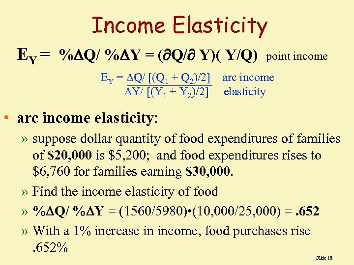Income Elasticity EY = % Q/ % Y = ( Q/ Y)( Y/Q) point income EY = Q/ [(Q 1 + Q 2)/2] arc income Y/ [(Y 1 + Y 2)/2] elasticity • arc income elasticity: » suppose dollar quantity of food expenditures of families of $20, 000 is $5, 200; and food expenditures rises to $6, 760 for families earning $30, 000. » Find the income elasticity of food » % Q/ % Y = (1560/5980) • (10, 000/25, 000) =. 652 » With a 1% increase in income, food purchases rise. 652% Slide 18

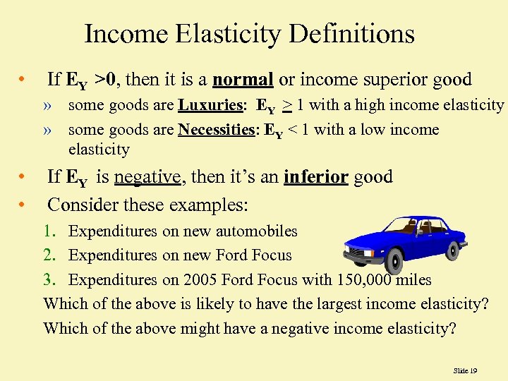Income Elasticity Definitions • If EY >0, then it is a normal or income superior good » some goods are Luxuries: EY > 1 with a high income elasticity » some goods are Necessities: EY < 1 with a low income elasticity • • If EY is negative, then it’s an inferior good Consider these examples: 1. Expenditures on new automobiles 2. Expenditures on new Ford Focus 3. Expenditures on 2005 Ford Focus with 150, 000 miles Which of the above is likely to have the largest income elasticity? Which of the above might have a negative income elasticity? Slide 19

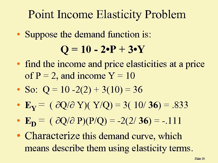Point Income Elasticity Problem • Suppose the demand function is: Q = 10 - 2 • P + 3 • Y • find the income and price elasticities at a price of P = 2, and income Y = 10 • So: Q = 10 -2(2) + 3(10) = 36 • EY = ( Q/ Y)( Y/Q) = 3( 10/ 36) =. 833 • ED = ( Q/ P)(P/Q) = -2(2/ 36) = -. 111 • Characterize this demand curve, which means describe them using elasticity terms. Slide 20

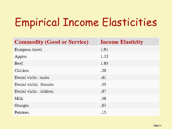Empirical Income Elasticities Commodity (Good or Service) Income Elasticity European travel 1. 91 Apples 1. 32 Beef 1. 05 Chicken . 28 Dental visits: males . 61 Dental visits|: females . 55 Dental visits: children . 87 Milk . 50 Oranges . 83 Potatoes . 15 Slide 21

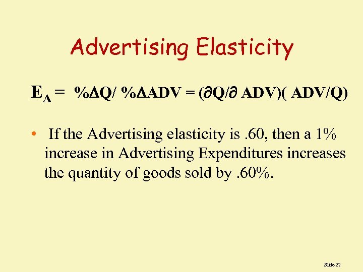Advertising Elasticity EA = % Q/ % ADV = ( Q/ ADV)( ADV/Q) • If the Advertising elasticity is. 60, then a 1% increase in Advertising Expenditures increases the quantity of goods sold by. 60%. Slide 22

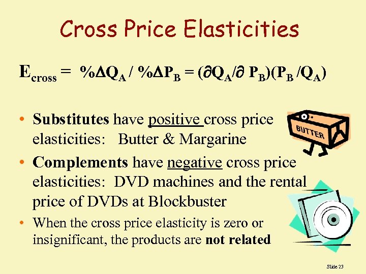Cross Price Elasticities Ecross = % QA / % PB = ( QA/ PB)(PB /QA) • Substitutes have positive cross price elasticities: Butter & Margarine • Complements have negative cross price elasticities: DVD machines and the rental price of DVDs at Blockbuster • When the cross price elasticity is zero or insignificant, the products are not related Slide 23

Antitrust & Cross Price Elasticities • Whether a product is a monopoly or in a larger industry is dependent on the closeness of the substitutes • Du. Pont’s cellophane was at first viewed as a monopoly. Economists showed that the cross price elasticity with other products such as aluminum foil, waxed paper, and other flexible wrapping paper was Positive, the large, Du. Pont showed its cellophane was not a monopoly in this larger market. Slide 24

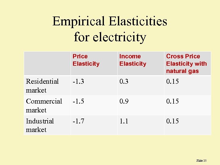Empirical Elasticities for electricity Price Elasticity Income Elasticity Cross Price Elasticity with natural gas Residential market -1. 3 0. 15 Commercial market -1. 5 0. 9 0. 15 Industrial market -1. 7 1. 1 0. 15 Slide 25

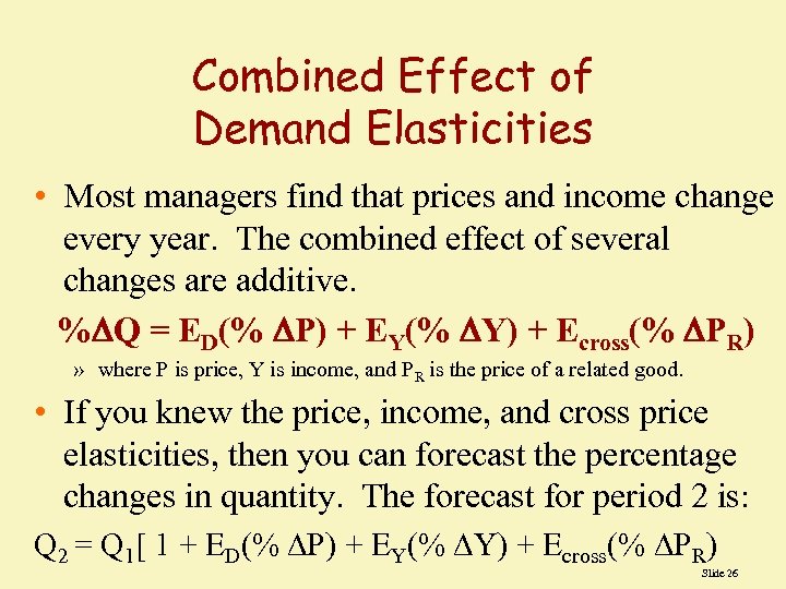Combined Effect of Demand Elasticities • Most managers find that prices and income change every year. The combined effect of several changes are additive. % Q = ED(% P) + EY(% Y) + Ecross(% PR) » where P is price, Y is income, and PR is the price of a related good. • If you knew the price, income, and cross price elasticities, then you can forecast the percentage changes in quantity. The forecast for period 2 is: Q 2 = Q 1[ 1 + ED(% P) + EY(% Y) + Ecross(% PR) Slide 26

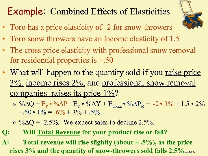Example: Combined Effects of Elasticities • Toro has a price elasticity of -2 for snow-throwers • Toro snow throwers have an income elasticity of 1. 5 • The cross price elasticity with professional snow removal for residential properties is +. 50 • What will happen to the quantity sold if you raise price 3%, income rises 2%, and professional snow removal companies raises its price 1%? » % Q = EP • % P +EY • % Y + Ecross • % PR = -2 • 3% + 1. 5 • 2% +. 50 • 1% = -6% + 3% +. 5% » % Q = -2. 5%. We expect sales to decline 2. 5%. Q: Will Total Revenue for your product rise or fall? A: Total revenue will rise slightly (about +. 5%), as the price rises 3% and the quantity of snow-throwers sold falls 2. 5%. Slide 27