7628b28f8444c99a060452810798abb4.ppt
- Количество слайдов: 20
Defining Probabilities: Random Variables • Examples: – Out of 100 heart catheterization procedures performed at a local hospital each year, the probability that more than five of them will result in complications is _____ – Drywall anchors are sold in packs of 50 at the local hardware store. The probability that no more than 3 will be defective is _____ – In general, EGR 252 - 4 ______ 1
Discrete Random Variables • Example: – Look back at problem 3, page 46. Assume someone spends $75 to buy 3 envelopes. The sample space describing the presence of $10 bills (H) vs bills that are not $10 (N) is: _______________ – The random variable associated with this situation, X, reflects the outcome of the choice and can take on the values: _______________ EGR 252 - 4 2
Discrete Probability Distributions • The probability that there are no $10 in the group is P(X = 0) = __________ (recall results from last time) • The probability distribution associated with the number of $10 bills is given by: x 0 1 2 3 P(X = x) EGR 252 - 4 3
Another Example • Example 3. 3, pg 66 P(X = 0) = ___________ EGR 252 - 4 4
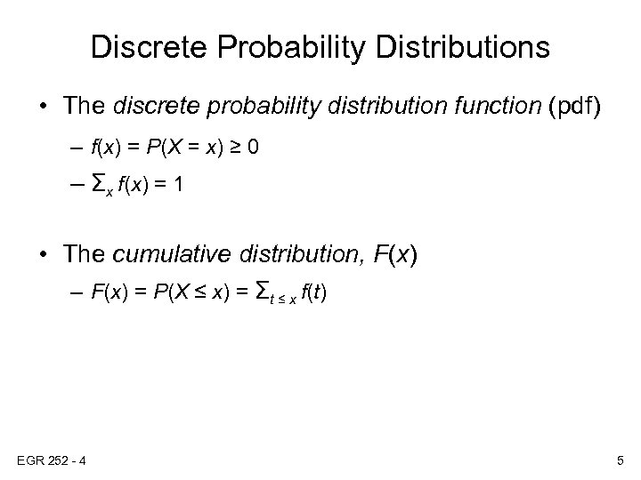
Discrete Probability Distributions • The discrete probability distribution function (pdf) – f(x) = P(X = x) ≥ 0 – Σx f(x) = 1 • The cumulative distribution, F(x) – F(x) = P(X ≤ x) = Σt ≤ x f(t) EGR 252 - 4 5
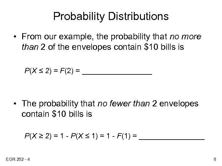
Probability Distributions • From our example, the probability that no more than 2 of the envelopes contain $10 bills is P(X ≤ 2) = F(2) = _________ • The probability that no fewer than 2 envelopes contain $10 bills is P(X ≥ 2) = 1 - P(X ≤ 1) = 1 - F(1) = ________ EGR 252 - 4 6
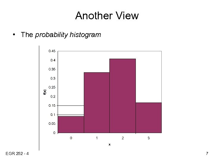
Another View • The probability histogram EGR 252 - 4 7
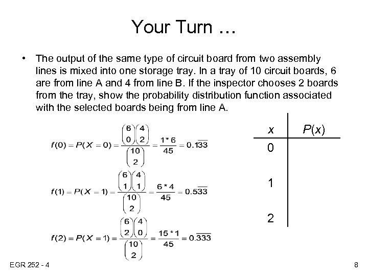
Your Turn … • The output of the same type of circuit board from two assembly lines is mixed into one storage tray. In a tray of 10 circuit boards, 6 are from line A and 4 from line B. If the inspector chooses 2 boards from the tray, show the probability distribution function associated with the selected boards being from line A. x 0 P(x) 1 2 EGR 252 - 4 8
Continuous Probability Distributions • Examples: – The probability that the average daily temperature in Georgia during the month of August falls between 90 and 95 degrees is _____ – The probability that a given part will fail before 1000 hours of use is _____ – In general, EGR 252 - 4 _____ 9
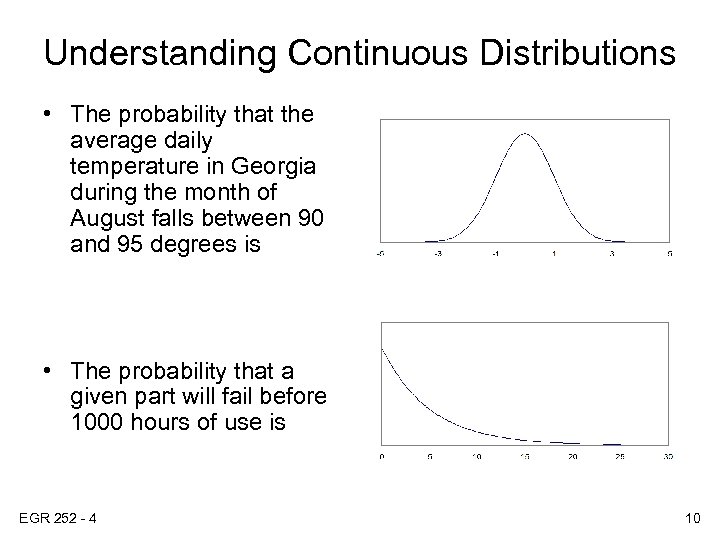
Understanding Continuous Distributions • The probability that the average daily temperature in Georgia during the month of August falls between 90 and 95 degrees is • The probability that a given part will fail before 1000 hours of use is EGR 252 - 4 10
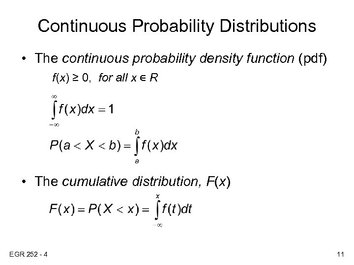
Continuous Probability Distributions • The continuous probability density function (pdf) f(x) ≥ 0, for all x ∈ R • The cumulative distribution, F(x) EGR 252 - 4 11
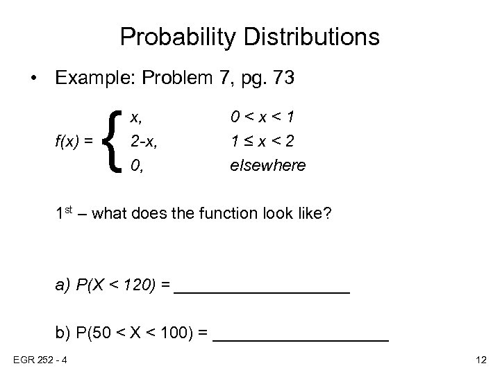
Probability Distributions • Example: Problem 7, pg. 73 f(x) = { x, 2 -x, 0, 0<x<1 1≤x<2 elsewhere 1 st – what does the function look like? a) P(X < 120) = __________ b) P(50 < X < 100) = __________ EGR 252 - 4 12
Your turn • Problem 14, pg. 73 EGR 252 - 4 13
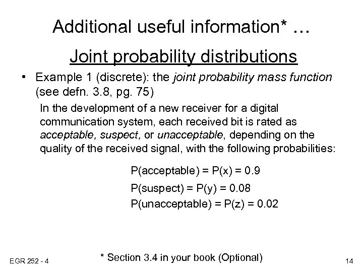
Additional useful information* … Joint probability distributions • Example 1 (discrete): the joint probability mass function (see defn. 3. 8, pg. 75) In the development of a new receiver for a digital communication system, each received bit is rated as acceptable, suspect, or unacceptable, depending on the quality of the received signal, with the following probabilities: P(acceptable) = P(x) = 0. 9 P(suspect) = P(y) = 0. 08 P(unacceptable) = P(z) = 0. 02 EGR 252 - 4 * Section 3. 4 in your book (Optional) 14
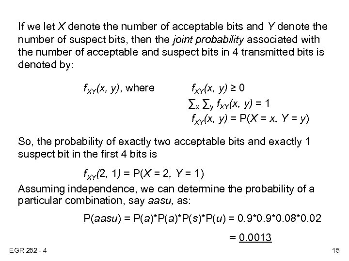
If we let X denote the number of acceptable bits and Y denote the number of suspect bits, then the joint probability associated with the number of acceptable and suspect bits in 4 transmitted bits is denoted by: f. XY(x, y), where f. XY(x, y) ≥ 0 ∑x ∑y f. XY(x, y) = 1 f. XY(x, y) = P(X = x, Y = y) So, the probability of exactly two acceptable bits and exactly 1 suspect bit in the first 4 bits is f. XY(2, 1) = P(X = 2, Y = 1) Assuming independence, we can determine the probability of a particular combination, say aasu, as: P(aasu) = P(a)*P(s)*P(u) = 0. 9*0. 08*0. 02 = 0. 0013 EGR 252 - 4 15
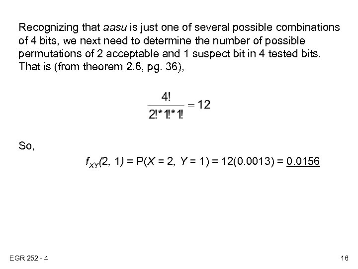
Recognizing that aasu is just one of several possible combinations of 4 bits, we next need to determine the number of possible permutations of 2 acceptable and 1 suspect bit in 4 tested bits. That is (from theorem 2. 6, pg. 36), So, f. XY(2, 1) = P(X = 2, Y = 1) = 12(0. 0013) = 0. 0156 EGR 252 - 4 16
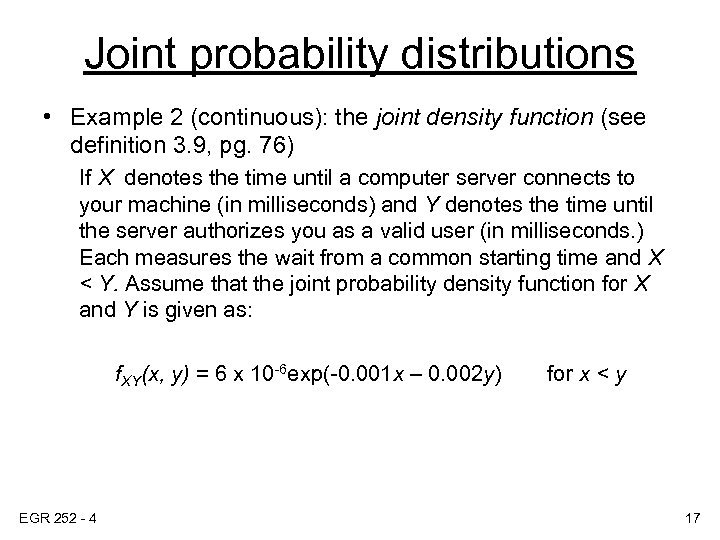
Joint probability distributions • Example 2 (continuous): the joint density function (see definition 3. 9, pg. 76) If X denotes the time until a computer server connects to your machine (in milliseconds) and Y denotes the time until the server authorizes you as a valid user (in milliseconds. ) Each measures the wait from a common starting time and X < Y. Assume that the joint probability density function for X and Y is given as: f. XY(x, y) = 6 x 10 -6 exp(-0. 001 x – 0. 002 y) EGR 252 - 4 for x < y 17
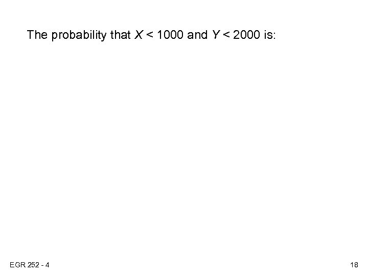
The probability that X < 1000 and Y < 2000 is: EGR 252 - 4 18
![[Note: we can verify that this density function integrates to 1 as follows: ] [Note: we can verify that this density function integrates to 1 as follows: ]](https://present5.com/presentation/7628b28f8444c99a060452810798abb4/image-19.jpg)
[Note: we can verify that this density function integrates to 1 as follows: ] EGR 252 - 4 19
For further study … • Read section 3. 4 • Solve selected problems on pp. 84 -86 EGR 252 - 4 20
7628b28f8444c99a060452810798abb4.ppt