DECISION MODELING WITH MICROSOFT EXCEL Chapter 13 Part

DECISION MODELING WITH MICROSOFT EXCEL Chapter 13 Part 1 Copyright 2001 Prentice Hall Publishers and Ardith E. Baker

Many important decisions made by individuals and organizations crucially depend on an assessment of the_____. There a few “____” sayings that illustrate the promise and frustration of forecasting: “It is difficult to_____, especially in regards to the future. ” “It isn’t difficult to forecast, just to forecast ______. ” “_______, if tortured enough, will confess to just about anything. ”

Economic forecasts_____ Government policies and business decisions Insurance companies’ ______decisions in mortgages and bonds Service industries’ (such as airlines, hotels, rental cars, cruise lines, etc. ) forecasts of _______as input for revenue management Forecasting is playing an increasingly important role in the________. There is clearly a steady _____in the use of quantitative forecasting models at many levels in industry and government. The many types of forecasting models will be distributed into two major techniques: ______and______

______forecasting models possess two important and attractive features: 1. They are expressed in mathematical ____. Thus, they establish an unambiguous record of how the forecast is made. 2. With the use of ________and computers, quantitative models can be based on an amazing quantity of data. Two types of quantitative forecasting models that will be discussed in the next two sections are: ____models and _____models

In a _______forecasting model, the forecast for the quantity of interest “rides piggyback” on another quantity or set of quantities. In other words, our ____of the value of one variable (or perhaps several variables) enables us to forecast the value of another______. In this model, let y denote the _____of some variable of interest and ^ denote a predicted or _____value for y that variable.

Then, in a causal model, ^ = f (x , … x ) y 1 2 n where f is a forecasting____, or function, and x 1, x 2 , … xi , is a set of variables In this representation, the x variables are often called _____variables, whereas y ^ the is dependent or _____variable. We either _______the independent variables in advance or can forecast them more easily than ^ y. Then the independent variables will be used in the forecasting model to forecast the _____ variable.

Companies often find by looking at past _____that their monthly sales are directly related to the monthly______, and thus figure that a good forecast could be made using next month’s GDP figure. The only problem is that this quantity is not _______, or it may just be a forecast and thus not a truly independent______. To use a causal forecasting model, requires two conditions: 1. There must be a ______between values of the independent and dependent variables such that the former provides ______about the latter.

2. The _______for the independent variables must be known and available to the forecaster at the ____the forecast is made. Simply because there is a mathematical relationship does not ______that there is really cause and effect. One commonly used approach in creating a causal forecasting model is called_______. CURVE FITTING: AN OIL COMPANY EXPANSION Consider an oil company that is planning to expand its _____of modern self-service gasoline stations.

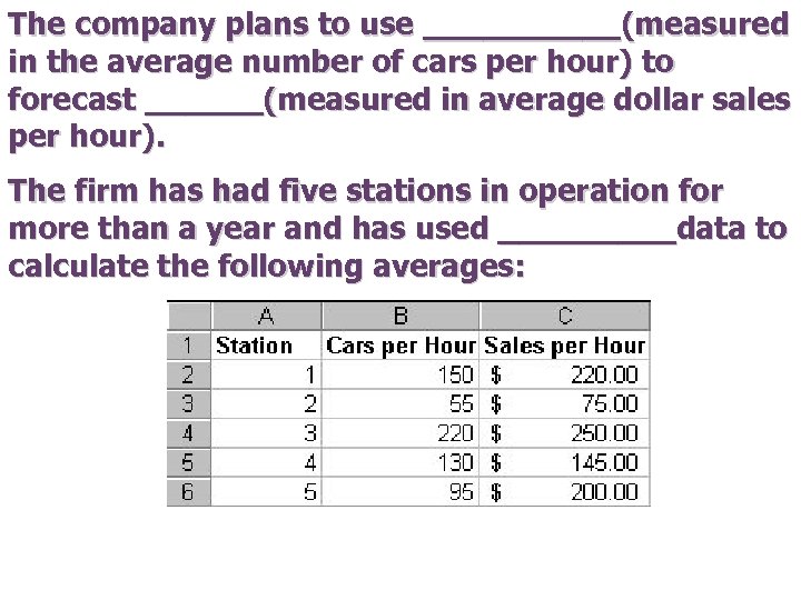The company plans to use _____(measured in the average number of cars per hour) to forecast ______(measured in average dollar sales per hour). The firm has had five stations in operation for more than a year and has used _____data to calculate the following averages:

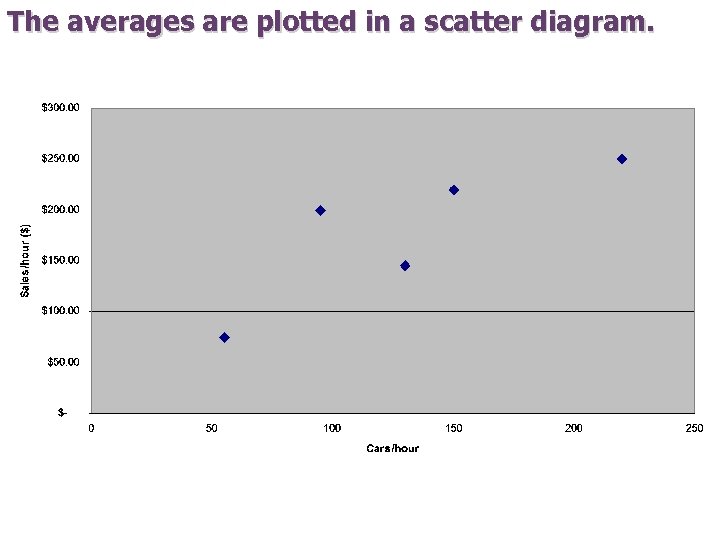The averages are plotted in a scatter diagram.

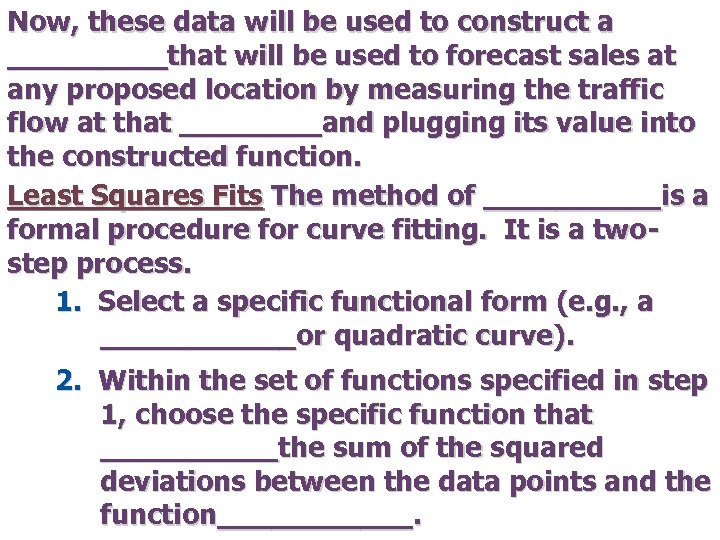Now, these data will be used to construct a _____that will be used to forecast sales at any proposed location by measuring the traffic flow at that ____and plugging its value into the constructed function. Least Squares Fits The method of _____is a formal procedure for curve fitting. It is a twostep process. 1. Select a specific functional form (e. g. , a ______or quadratic curve). 2. Within the set of functions specified in step 1, choose the specific function that _____the sum of the squared deviations between the data points and the function______.

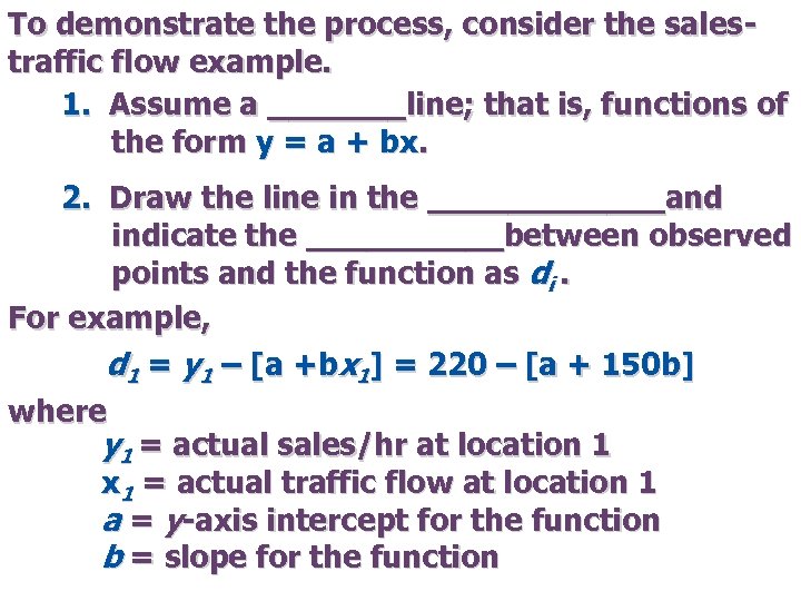To demonstrate the process, consider the salestraffic flow example. 1. Assume a _______line; that is, functions of the form y = a + bx. 2. Draw the line in the ______and indicate the _____between observed points and the function as di. For example, d 1 = y 1 – [a +bx 1] = 220 – [a + 150 b] where y 1 = actual sales/hr at location 1 x 1 = actual traffic flow at location 1 a = y-axis intercept for the function b = slope for the function

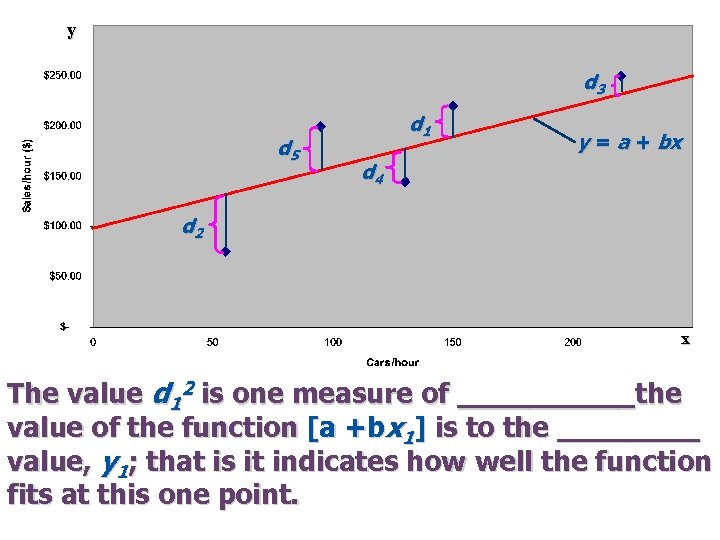y d 3 d 5 d 1 y = a + bx d 4 d 2 x The value d 12 is one measure of _____the value of the function [a +bx 1] is to the ____ value, y 1; that is it indicates how well the function fits at this one point.

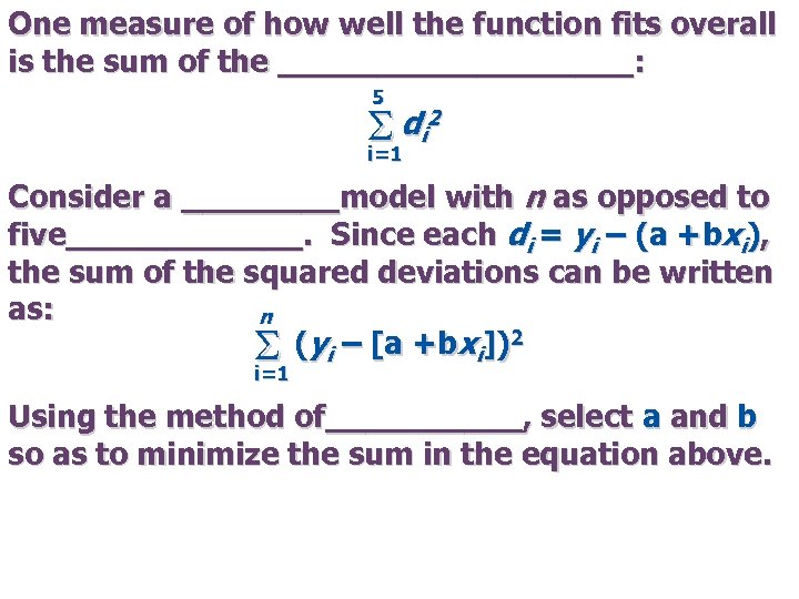One measure of how well the function fits overall is the sum of the _________: 5 S di 2 i=1 Consider a ____model with n as opposed to five______. Since each di = yi – (a +bxi), the sum of the squared deviations can be written as: n (yi – [a +bxi])2 S i=1 Using the method of_____, select a and b so as to minimize the sum in the equation above.

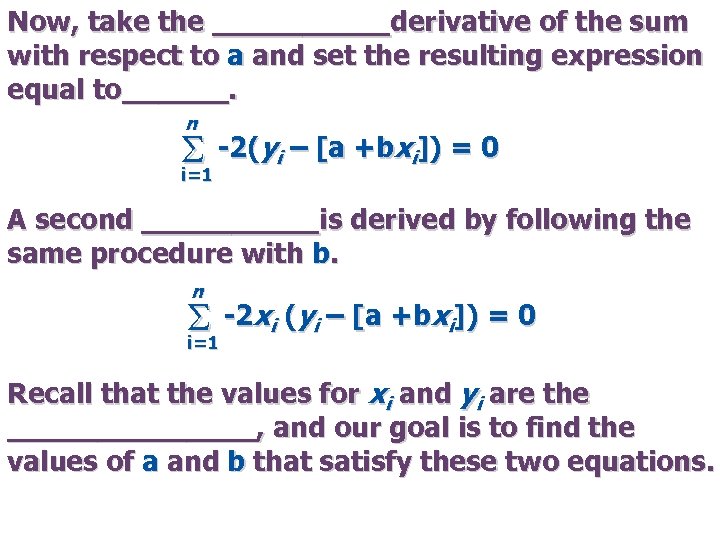Now, take the _____derivative of the sum with respect to a and set the resulting expression equal to______. n S -2(yi – [a +bxi]) = 0 i=1 A second _____is derived by following the same procedure with b. n S -2 xi (yi – [a +bxi]) = 0 i=1 Recall that the values for xi and yi are the _______, and our goal is to find the values of a and b that satisfy these two equations.

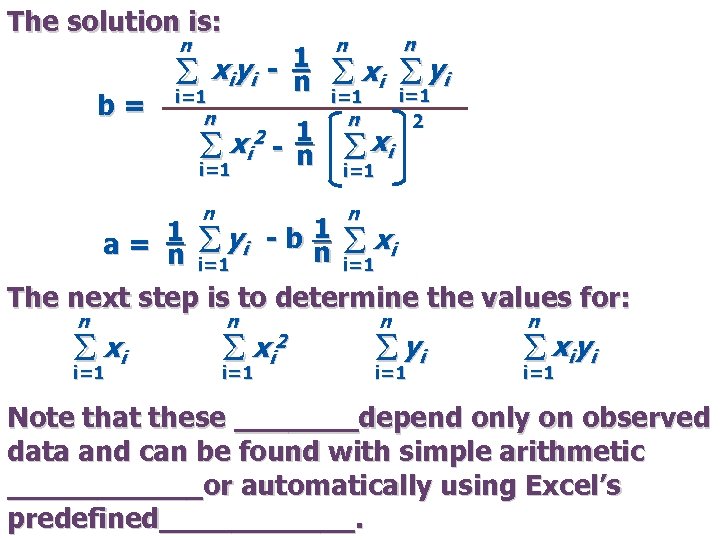The solution is: n b= xiy i - 1 S n i=1 n n n S xi S y i i=1 n xi 2 - 1 S n i=1 S xi i=1 n 2 n 1 Sy - b 1 S x a= n i=1 i i=1 The next step is to determine the values for: n S xi i=1 n S xi 2 i=1 n S yi i=1 n S xiy i i=1 Note that these _______depend only on observed data and can be found with simple arithmetic ______or automatically using Excel’s predefined______.

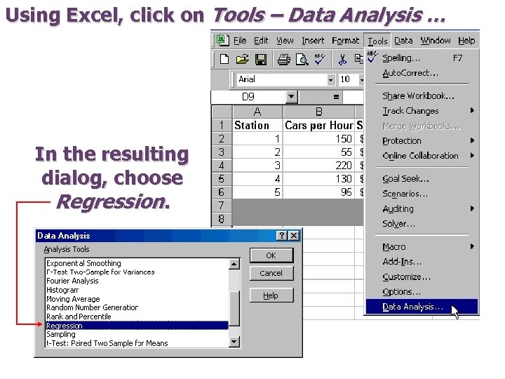Using Excel, click on Tools – Data Analysis … In the resulting dialog, choose Regression.

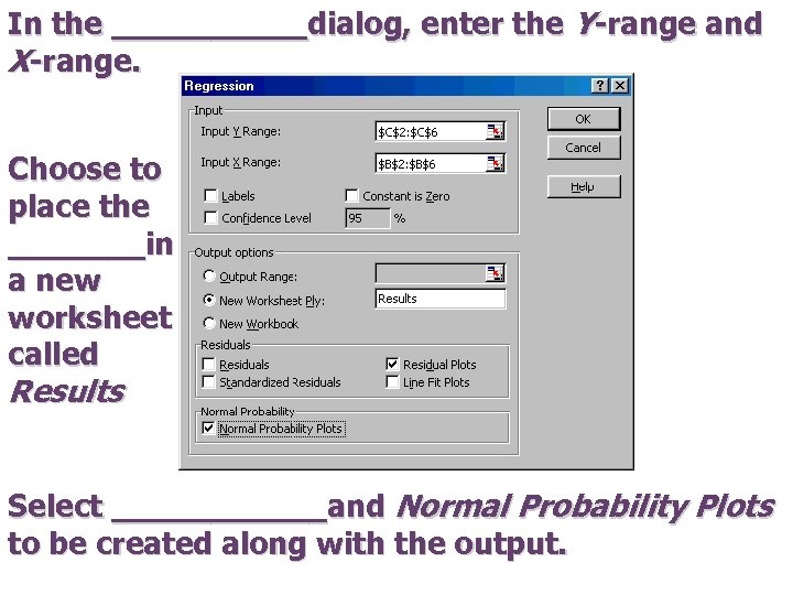In the _____dialog, enter the Y-range and X-range. Choose to place the _______in a new worksheet called Results Select ______and Normal Probability Plots to be created along with the output.

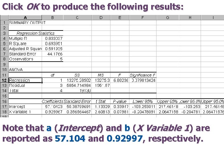Click OK to produce the following results: Note that a (Intercept) and b (X Variable 1) are reported as 57. 104 and 0. 92997, respectively.

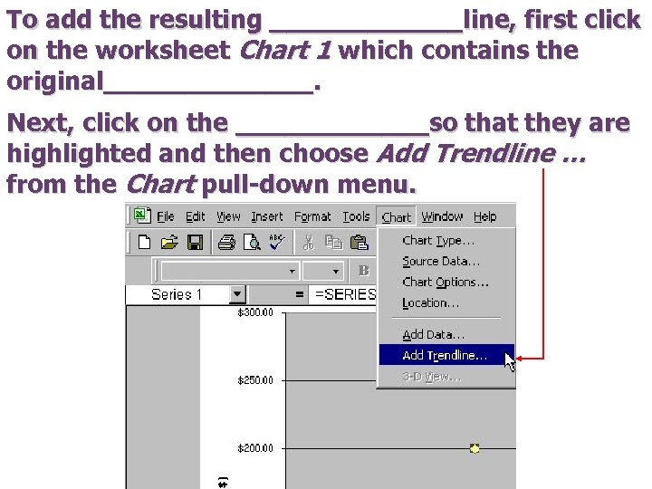To add the resulting ______line, first click on the worksheet Chart 1 which contains the original_______. Next, click on the ______so that they are highlighted and then choose Add Trendline … from the Chart pull-down menu.

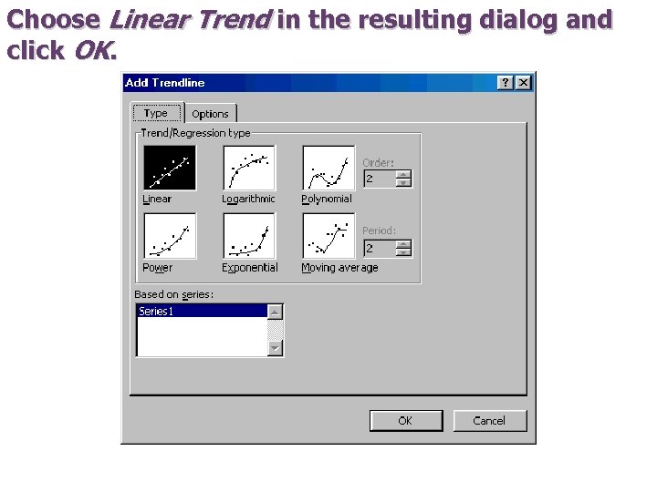Choose Linear Trend in the resulting dialog and click OK.

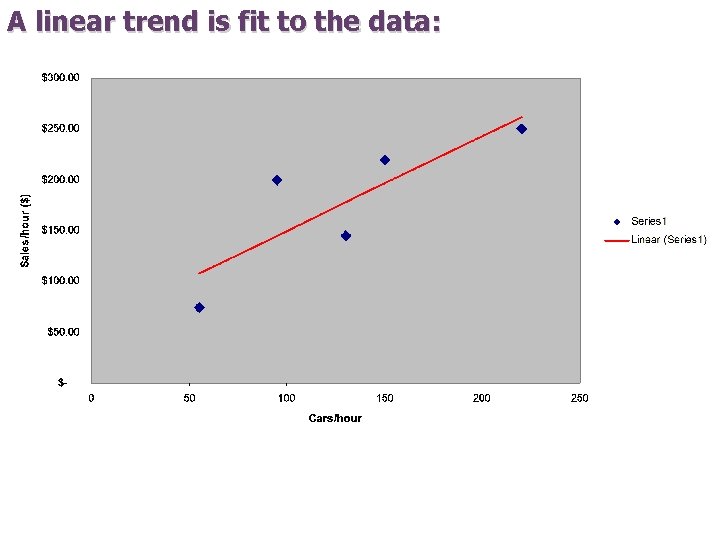A linear trend is fit to the data:

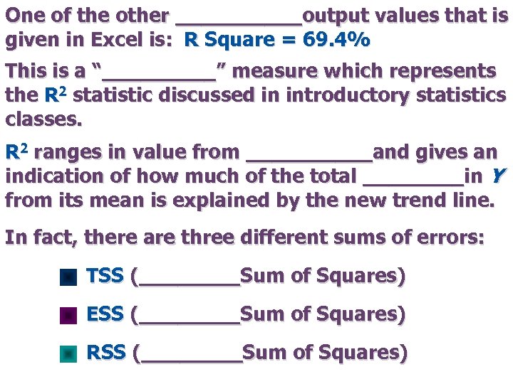One of the other _____output values that is given in Excel is: R Square = 69. 4% This is a “_____” measure which represents the R 2 statistic discussed in introductory statistics classes. R 2 ranges in value from _____and gives an indication of how much of the total ____in Y from its mean is explained by the new trend line. In fact, there are three different sums of errors: TSS (____Sum of Squares) ESS (____Sum of Squares) RSS (____Sum of Squares)

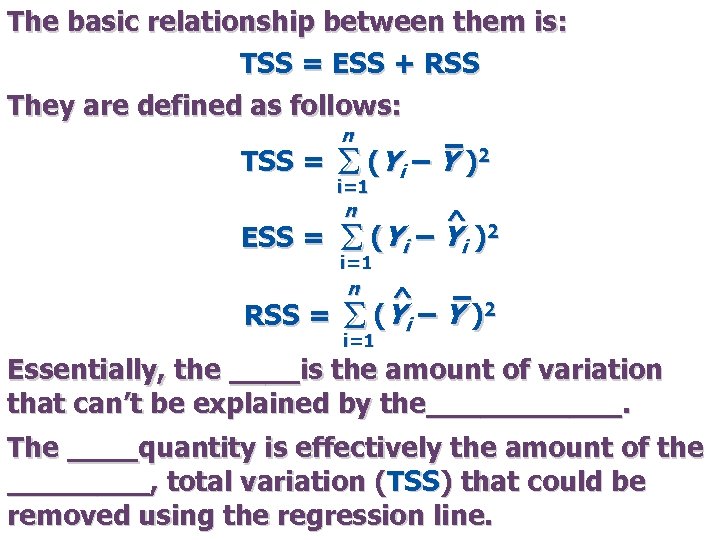The basic relationship between them is: TSS = ESS + RSS They are defined as follows: n – 2 TSS = S (Yi – Y ) i=1 ESS = n ^ S (Y i – Y i )2 i=1 n ^ – 2 RSS = S (Yi – Y ) i=1 Essentially, the ____is the amount of variation that can’t be explained by the______. The ____quantity is effectively the amount of the ____, total variation (TSS) that could be removed using the regression line.

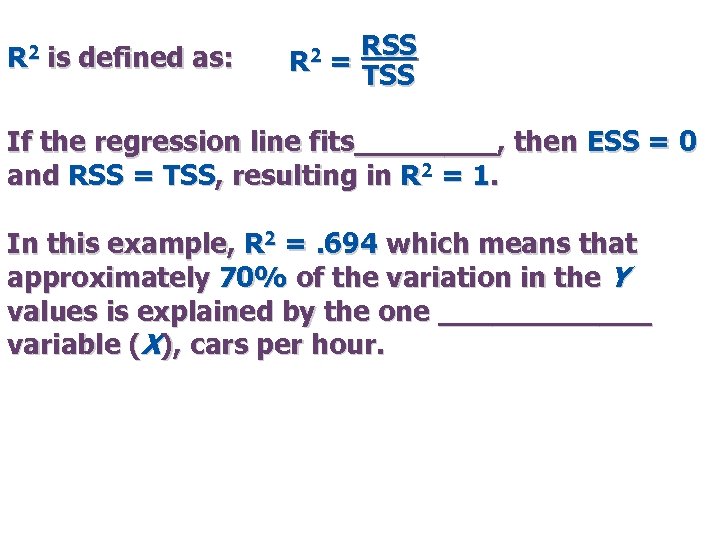R 2 is defined as: R 2 RSS = TSS If the regression line fits____, then ESS = 0 and RSS = TSS, resulting in R 2 = 1. In this example, R 2 =. 694 which means that approximately 70% of the variation in the Y values is explained by the one ______ variable (X), cars per hour.

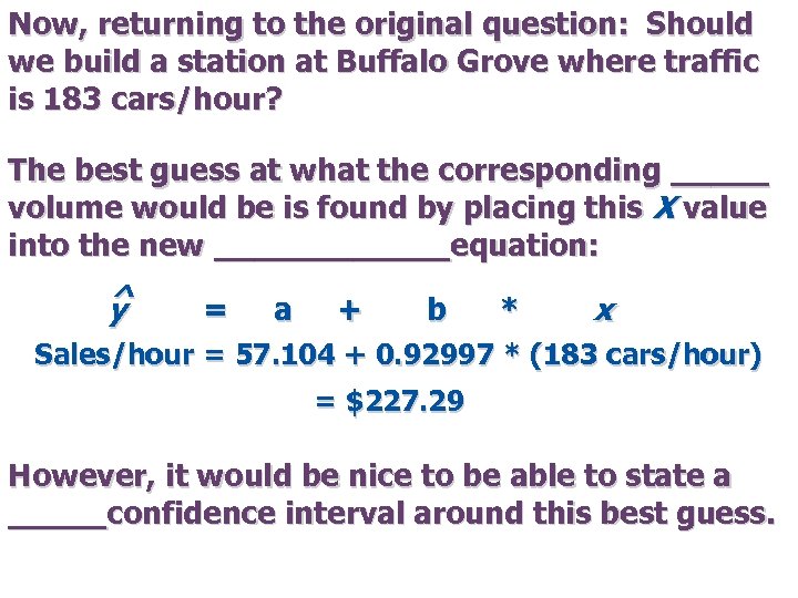Now, returning to the original question: Should we build a station at Buffalo Grove where traffic is 183 cars/hour? The best guess at what the corresponding _____ volume would be is found by placing this X value into the new ______equation: ^ y = a + b * x Sales/hour = 57. 104 + 0. 92997 * (183 cars/hour) = $227. 29 However, it would be nice to be able to state a _____confidence interval around this best guess.

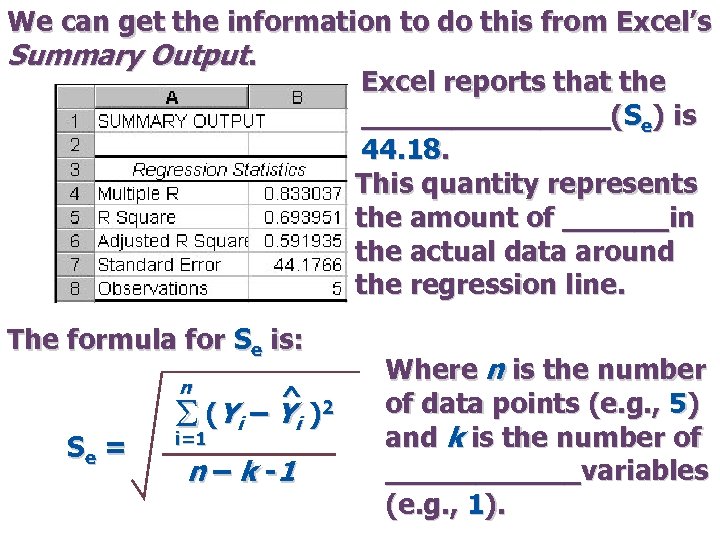We can get the information to do this from Excel’s Summary Output. Excel reports that the _______(Se) is 44. 18. This quantity represents the amount of ______in the actual data around the regression line. The formula for Se is: n Se = ^ S (Y i – Y i )2 i=1 n – k -1 Where n is the number of data points (e. g. , 5) and k is the number of ______variables (e. g. , 1).

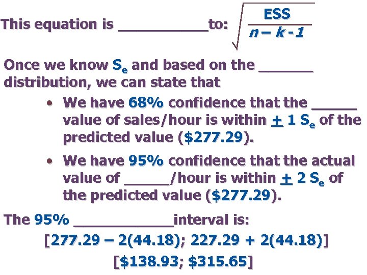This equation is _____to: ESS n – k -1 Once we know Se and based on the ______ distribution, we can state that • We have 68% confidence that the _____ value of sales/hour is within + 1 Se of the predicted value ($277. 29). • We have 95% confidence that the actual value of _____/hour is within + 2 Se of the predicted value ($277. 29). The 95% ______interval is: [277. 29 – 2(44. 18); 227. 29 + 2(44. 18)] [$138. 93; $315. 65]

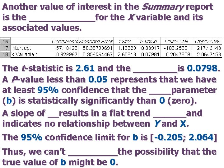Another value of interest in the Summary report is the ______for the X variable and its associated values. The t-statistic is 2. 61 and the ____is 0. 0798. A P-value less than 0. 05 represents that we have at least 95% confidence that the ____parameter (b) is statistically significantly than 0 (zero). A slope of __results in a flat trend ______and indicates no relationship between Y and X. The 95% confidence limit for b is [-0. 205; 2. 064] Thus, we can’t _____the possibility that the true value of b might be 0.

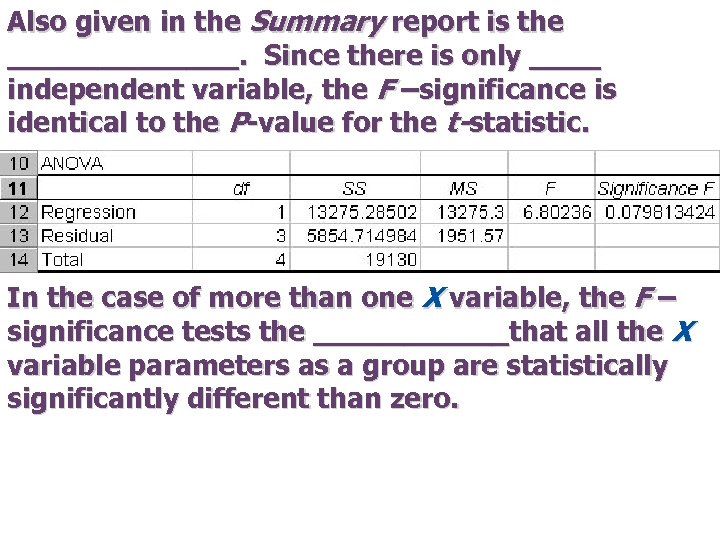Also given in the Summary report is the _______. Since there is only ____ independent variable, the F –significance is identical to the P-value for the t-statistic. In the case of more than one X variable, the F – significance tests the ______that all the X variable parameters as a group are statistically significantly different than zero.

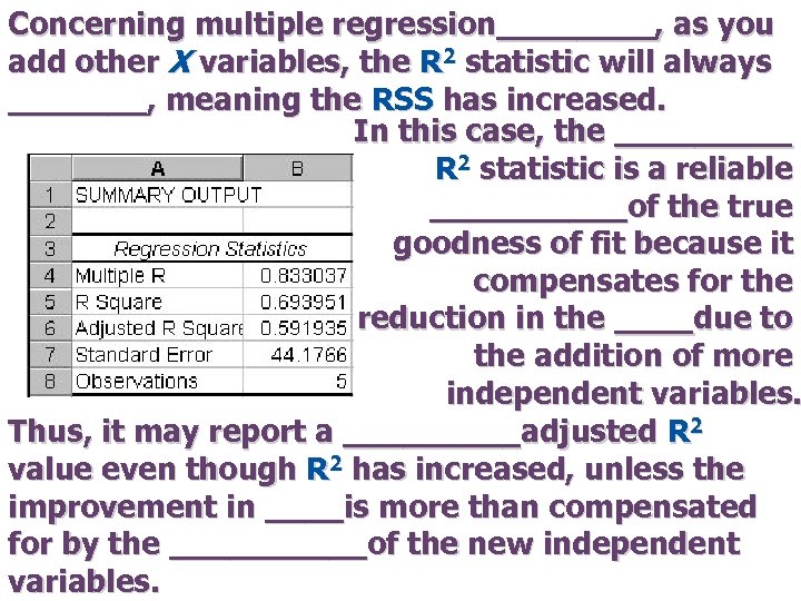Concerning multiple regression____, as you add other X variables, the R 2 statistic will always _______, meaning the RSS has increased. In this case, the _____ R 2 statistic is a reliable _____of the true goodness of fit because it compensates for the reduction in the ____due to the addition of more independent variables. Thus, it may report a _____adjusted R 2 value even though R 2 has increased, unless the improvement in ____is more than compensated for by the _____of the new independent variables.

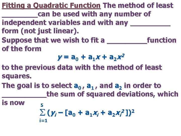Fitting a Quadratic Function The method of least ____can be used with any number of independent variables and with any _____ form (not just linear). Suppose that we wish to fit a _____function of the form y = a 0 + a 1 x + a 2 x 2 to the previous data with the method of least squares. The goal is to select a 0 , a 1 , and a 2 in order to _____the sum of squared deviations, which is now 5 S (yi – [a 0 + a 1 xi + a 2 xi 2 ])2 i=1

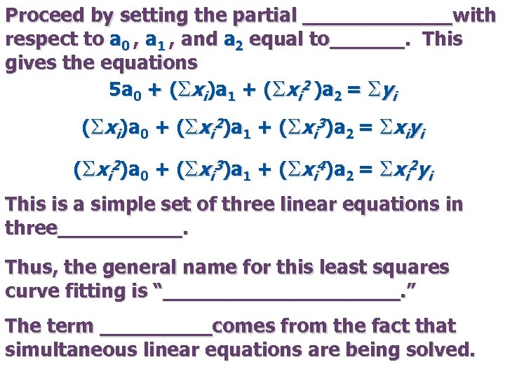Proceed by setting the partial ______with respect to a 0 , a 1 , and a 2 equal to______. This gives the equations 5 a 0 + (Sxi)a 1 + (Sxi 2 )a 2 = Syi (Sxi)a 0 + (Sxi 2)a 1 + (Sxi 3)a 2 = Sxiyi (Sxi 2)a 0 + (Sxi 3)a 1 + (Sxi 4)a 2 = Sxi 2 yi This is a simple set of three linear equations in three_____. Thus, the general name for this least squares curve fitting is “__________. ” The term _____comes from the fact that simultaneous linear equations are being solved.

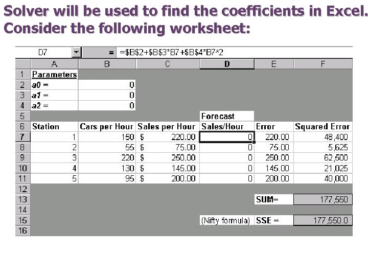Solver will be used to find the coefficients in Excel. Consider the following worksheet:

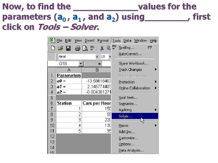Now, to find the ______values for the parameters (a 0 , a 1 , and a 2) using____, first click on Tools – Solver.

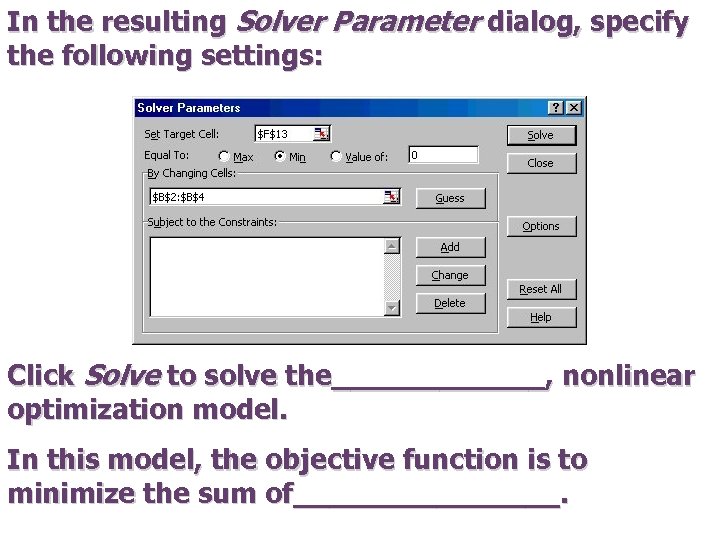In the resulting Solver Parameter dialog, specify the following settings: Click Solve to solve the______, nonlinear optimization model. In this model, the objective function is to minimize the sum of________.

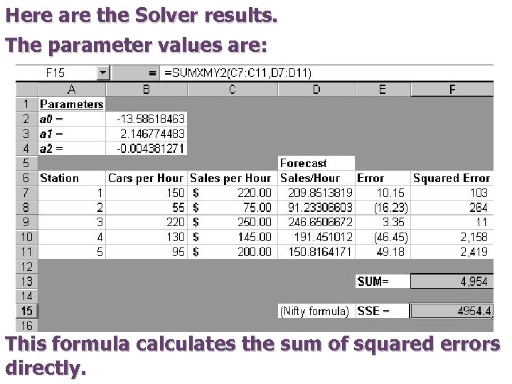Here are the Solver results. The parameter values are: This formula calculates the sum of squared errors directly.

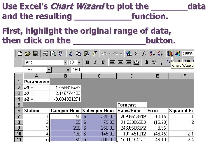Use Excel’s Chart Wizard to plot the _______data and the resulting ______function. First, highlight the original range of data, then click on the _______button.

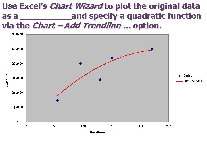Use Excel’s Chart Wizard to plot the original data as a _____and specify a quadratic function via the Chart – Add Trendline … option.

Comparing the Linear and Quadratic Fits In the method of least squares, the _____of the squared deviations was selected as the measure of “_______. ” Thus, the linear and quadratic fits can be compared with this______. In order to make this comparison, go back to the linear regression “____” spreadsheet and make the corresponding calculation in the original “______” spreadsheet.

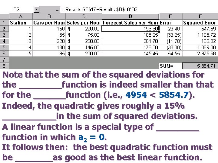Note that the sum of the squared deviations for the ____function is indeed smaller than that for the ______function (i. e. , 4954 < 5854. 7). Indeed, the quadratic gives roughly a 15% _____in the sum of squared deviations. A linear function is a special type of ____ function in which a 2 = 0. It follows then: the best quadratic function must be _______as good as the best linear function.

WHICH CURVE TO FIT? If a quadratic function is at least as good as a linear function, why not choose a more ____ form, thereby getting an even better_____? In practice, _______of the form (with only a single independent variable for illustrative purposes) are often suggested: y = a 0 + a 1 x + a 2 x 2 + … + a nx n Such a function is called a _____of degree n, and it represents a broad and flexible class of functions. n=2 quadratic n=3 cubic n=4 _______ …

One must proceed with _____when fitting data with a ______function. For example, it is possible to find a (k – 1)-degree polynomial that will _____fit k data points. To be more specific, suppose we have seven _____observations, denoted (xi , yi), i = 1, 2, …, 7 It is possible to find a ______polynomial y = a 0 + a 1 x + a 2 x 2 + … + a 6 x 6 that exactly passes through each of these seven data points.

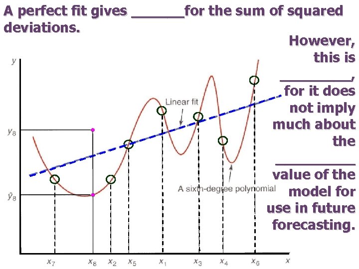A perfect fit gives ______for the sum of squared deviations. However, this is ____, for it does not imply much about the _____ value of the model for use in future forecasting.

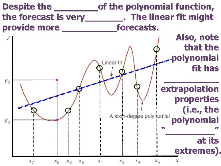Despite the ____of the polynomial function, the forecast is very_______. The linear fit might provide more _____forecasts. Also, note that the polynomial fit has _____ extrapolation properties (i. e. , the polynomial “_____” at its extremes).

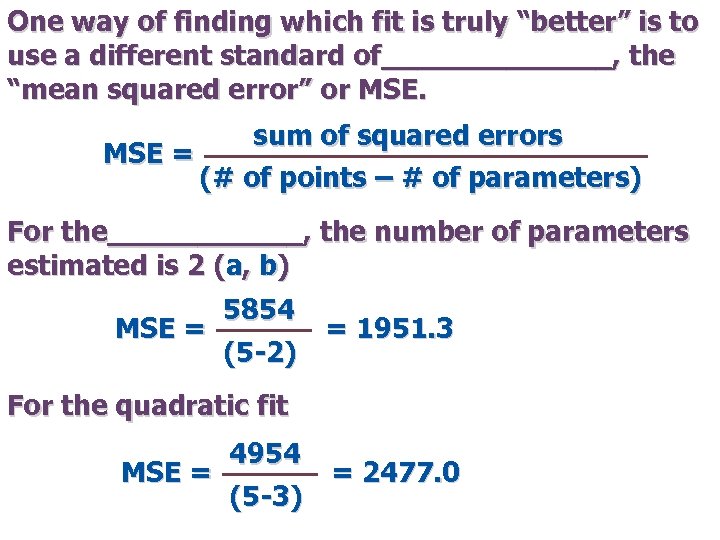One way of finding which fit is truly “better” is to use a different standard of_______, the “mean squared error” or MSE. sum of squared errors MSE = (# of points – # of parameters) For the______, the number of parameters estimated is 2 (a, b) 5854 MSE = = 1951. 3 (5 -2) For the quadratic fit 4954 MSE = = 2477. 0 (5 -3)

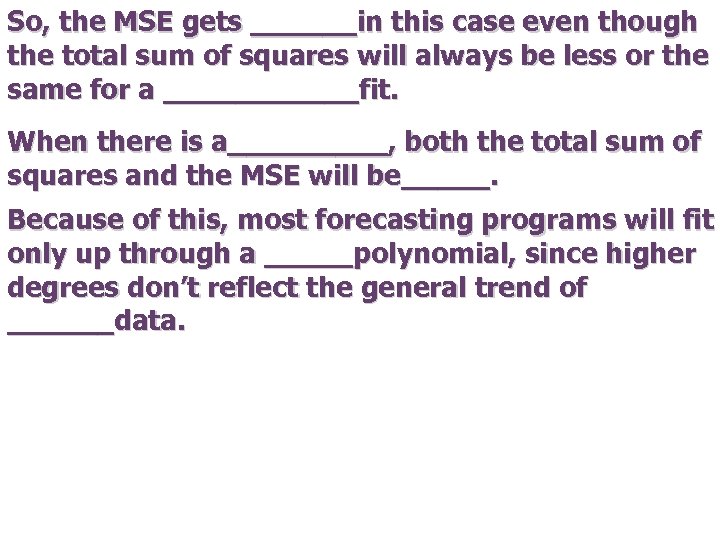So, the MSE gets ______in this case even though the total sum of squares will always be less or the same for a ______fit. When there is a_____, both the total sum of squares and the MSE will be_____. Because of this, most forecasting programs will fit only up through a _____polynomial, since higher degrees don’t reflect the general trend of ______data.

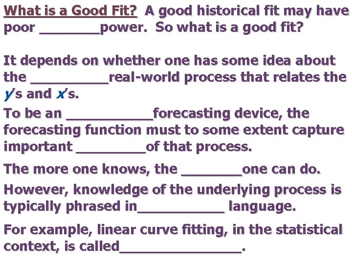What is a Good Fit? A good historical fit may have poor _______power. So what is a good fit? It depends on whether one has some idea about the _____real-world process that relates the y’s and x’s. To be an _____forecasting device, the forecasting function must to some extent capture important ____of that process. The more one knows, the _______one can do. However, knowledge of the underlying process is typically phrased in_____ language. For example, linear curve fitting, in the statistical context, is called_______.

If the statistical _______about the linear regression model are precisely satisfied (e. g. , errors are _____distributed around the regression line), then in a precise and welldefined sense, statisticians can prove that the linear fit is the “______possible fit. ” In the real world one can never be completely certain about the ______process. The question then becomes: How much ______can we have that the underlying process is one that satisfies a particular set of statistical______? Fortunately, statistical analysis can reveal how well the _____data do indeed satisfy those assumptions.

And if it does not satisfy the assumptions, then try a different____. Remember, there is an underlying real-world _____and the model is a selective __________of that problem. How good is that model? Ideally, to test the goodness of a model, one would like to have considerable ______with its use. If, in repeated use, it is observed that the model performs well, then our confidence is____. However, what confidence can we have at the outset, without experience?

Validating Models One_____, is to ask the question: Suppose the model had been used to make past decisions; how well would the firm have fared? This approach “creates” experience by ____ the past. This is often referred to as _____of the model. Typically, one uses only a ______of the historical data to create the model – for example, to fit a polynomial of a specified degree. One can then use the remaining _____to see how well the model would have performed.

End of Part 1 Please continue to Part 2