Decision Making Under Uncertainty Lec 9 Approximate Value

Decision Making Under Uncertainty Lec #9: Approximate Value Function UIUC CS 598: Section EA Professor: Eyal Amir Spring Semester 2006 Some slides by Jeremy Wyatt (U Birmingham), Ron Parr (Duke), Eduardo Alonso, and Craig Boutilier (Toronto)

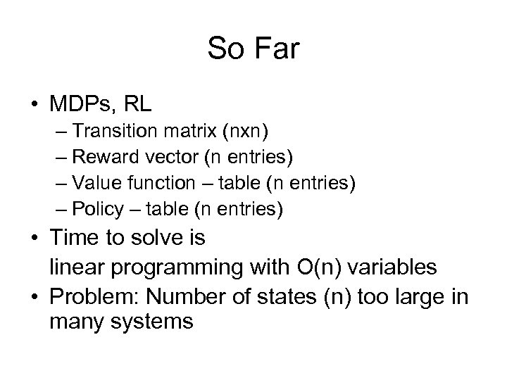So Far • MDPs, RL – Transition matrix (nxn) – Reward vector (n entries) – Value function – table (n entries) – Policy – table (n entries) • Time to solve is linear programming with O(n) variables • Problem: Number of states (n) too large in many systems

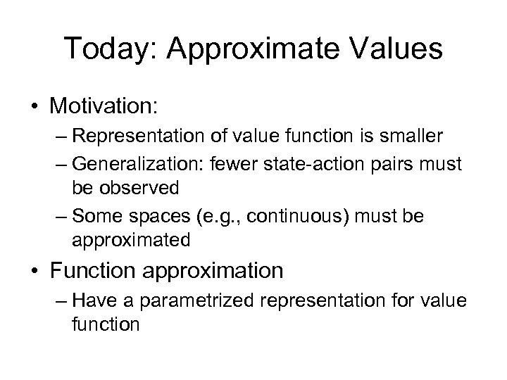Today: Approximate Values • Motivation: – Representation of value function is smaller – Generalization: fewer state-action pairs must be observed – Some spaces (e. g. , continuous) must be approximated • Function approximation – Have a parametrized representation for value function

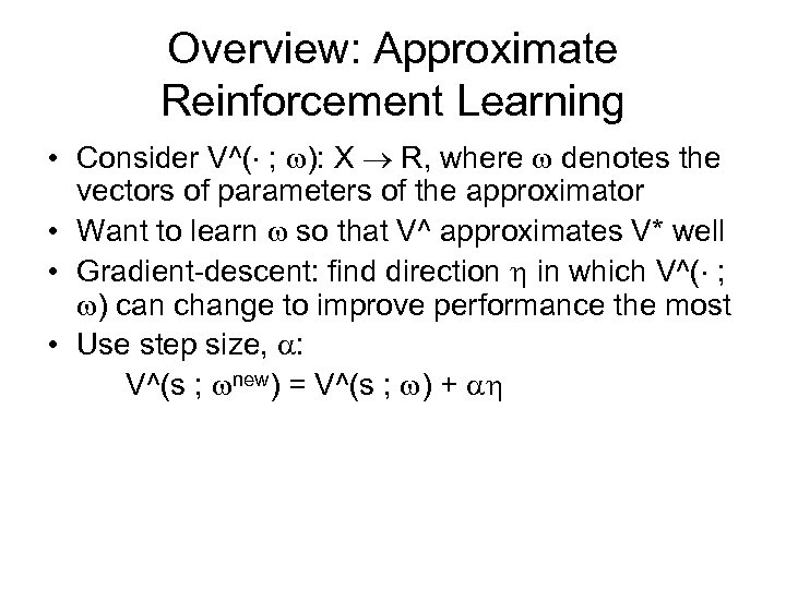Overview: Approximate Reinforcement Learning • Consider V^( ; ): X R, where denotes the vectors of parameters of the approximator • Want to learn so that V^ approximates V* well • Gradient-descent: find direction in which V^( ; ) can change to improve performance the most • Use step size, : V^(s ; new) = V^(s ; ) +

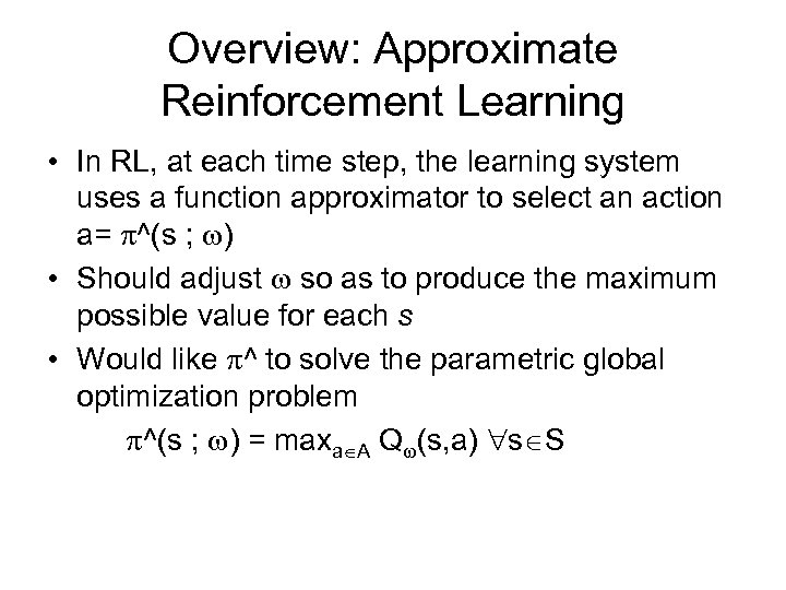Overview: Approximate Reinforcement Learning • In RL, at each time step, the learning system uses a function approximator to select an action a= ^(s ; ) • Should adjust so as to produce the maximum possible value for each s • Would like ^ to solve the parametric global optimization problem ^(s ; ) = maxa A Q (s, a) s S

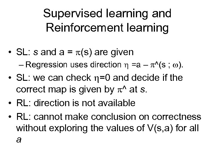Supervised learning and Reinforcement learning • SL: s and a = (s) are given – Regression uses direction =a – ^(s ; ). • SL: we can check =0 and decide if the correct map is given by ^ at s. • RL: direction is not available • RL: cannot make conclusion on correctness without exploring the values of V(s, a) for all a

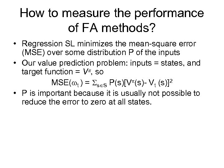How to measure the performance of FA methods? • Regression SL minimizes the mean-square error (MSE) over some distribution P of the inputs • Our value prediction problem: inputs = states, and target function = V , so MSE( t ) = s S P(s)[V (s)- Vt (s)]2 • P is important because it is usually not possible to reduce the error to zero at all states.

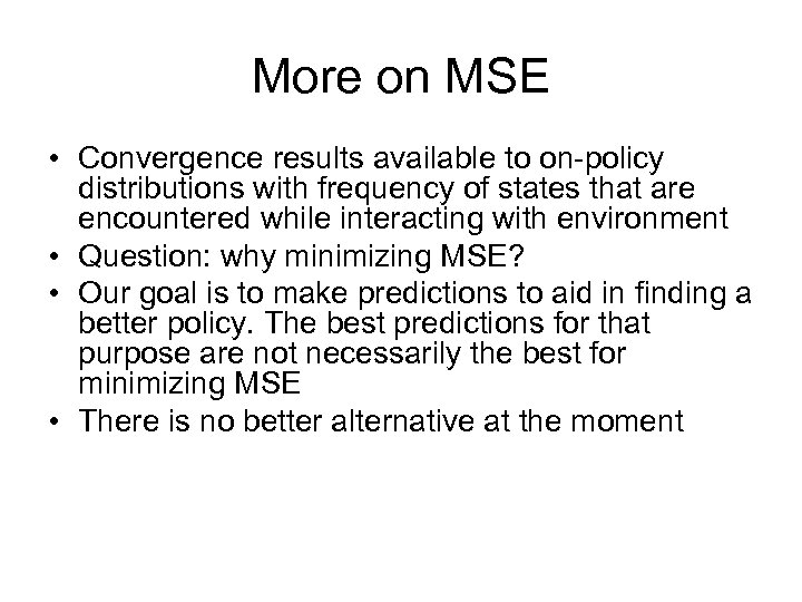More on MSE • Convergence results available to on-policy distributions with frequency of states that are encountered while interacting with environment • Question: why minimizing MSE? • Our goal is to make predictions to aid in finding a better policy. The best predictions for that purpose are not necessarily the best for minimizing MSE • There is no better alternative at the moment

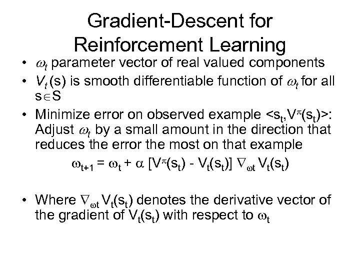Gradient-Descent for Reinforcement Learning • t parameter vector of real valued components • Vt (s) is smooth differentiable function of t for all s S • Minimize error on observed example : Adjust t by a small amount in the direction that reduces the error the most on that example t+1 = t + [V (st) - Vt(st)] t Vt(st) • Where t Vt(st) denotes the derivative vector of the gradient of Vt(st) with respect to t

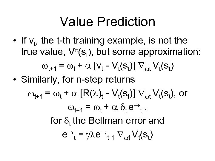Value Prediction • If vt, the t-th training example, is not the true value, V (st), but some approximation: t+1 = t + [vt - Vt(st)] t Vt(st) • Similarly, for n-step returns t+1 = t + [R( )t - Vt(st)] t Vt(st), or t+1 = t + t e t , for t the Bellman error and e t = e t-1 t Vt(st)

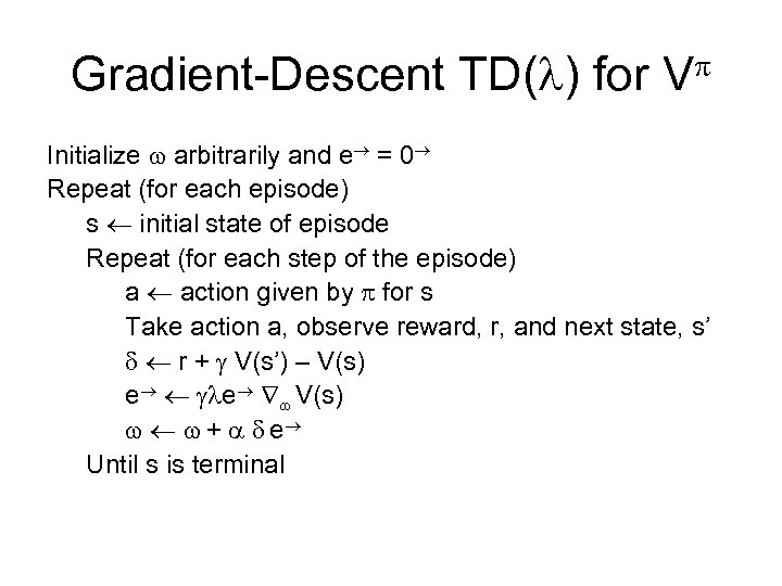Gradient-Descent TD( ) for V Initialize arbitrarily and e = 0 Repeat (for each episode) s initial state of episode Repeat (for each step of the episode) a action given by for s Take action a, observe reward, r, and next state, s’ r + V(s’) – V(s) e e V(s) + e Until s is terminal

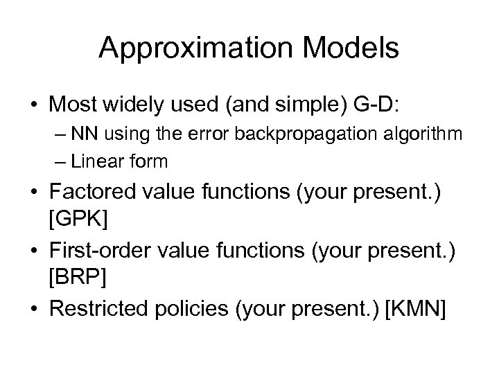Approximation Models • Most widely used (and simple) G-D: – NN using the error backpropagation algorithm – Linear form • Factored value functions (your present. ) [GPK] • First-order value functions (your present. ) [BRP] • Restricted policies (your present. ) [KMN]

Approximation Models • Most widely used (and simple) G-D: – NN using the error backpropagation algorithm – Linear form • Factored value functions (your present. ) [GPK] • First-order value functions (your present. ) [BRP] • Restricted policies (your present. ) [KMN]

Function Approximation • Common approach to solving MDPs – find a functional form f(q) for VF that is tractable • e. g. , not exponential in number of variables – attempt to find parameters q s. t. f(q) offers “best fit” to “true” VF • Example: – use neural net to approximate VF • inputs: state features; output: value or Q-value – generate samples of “true VF” to train NN • e. g. , use dynamics to sample transitions and train on Bellman backups (bootstrap on current approximation given by NN)

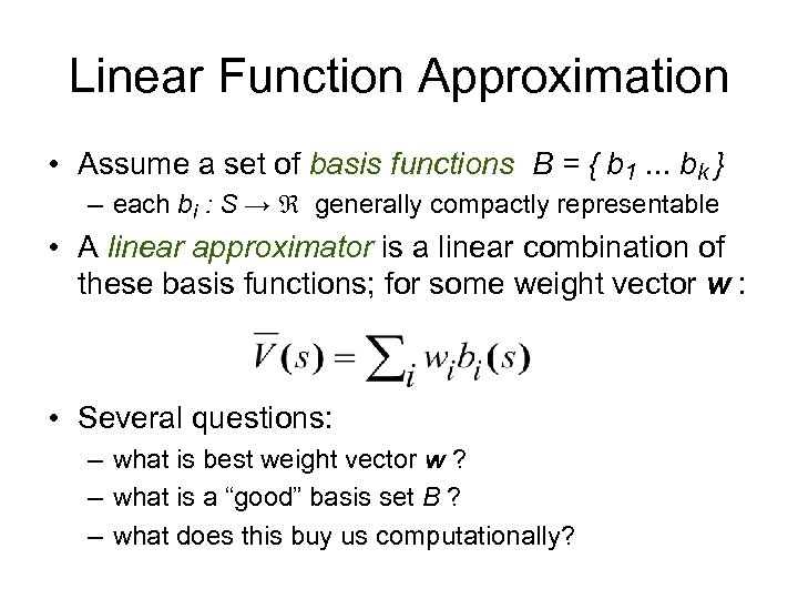Linear Function Approximation • Assume a set of basis functions B = { b 1. . . bk } – each bi : S → generally compactly representable • A linear approximator is a linear combination of these basis functions; for some weight vector w : • Several questions: – what is best weight vector w ? – what is a “good” basis set B ? – what does this buy us computationally?

Flexibility of Linear Decomposition • Assume each basis function is compact – e. g. , refers only a few vars; b 1(X, Y), b 2(W, Z), b 3(A) • Then VF is compact: – V(X, Y, W, Z, A) = w 1 b 1(X, Y) + w 2 b 2(W, Z) + w 3 b 3(A) • For given representation size (10 parameters), we get more value flexibility (32 distinct values) compared to a piecewise constant rep’n

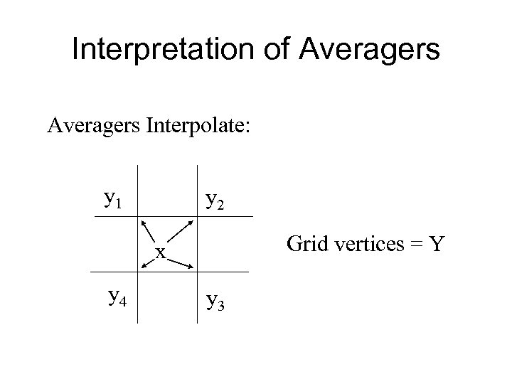Interpretation of Averagers Interpolate: y 1 y 2 Grid vertices = Y x y 4 y 3

Linear methods? • So, if we can find good basis sets (that allow a good fit), VF can be more compact • Several have been proposed: coarse coding, tile coding, radial basis functions, factored (project on a few variables), feature selection, first-order

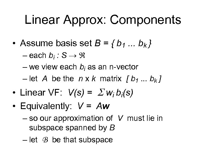Linear Approx: Components • Assume basis set B = { b 1. . . bk } – each bi : S → – we view each bi as an n-vector – let A be the n x k matrix [ b 1. . . bk ] • Linear VF: V(s) = S wi bi(s) • Equivalently: V = Aw – so our approximation of V must lie in subspace spanned by B – let B be that subspace

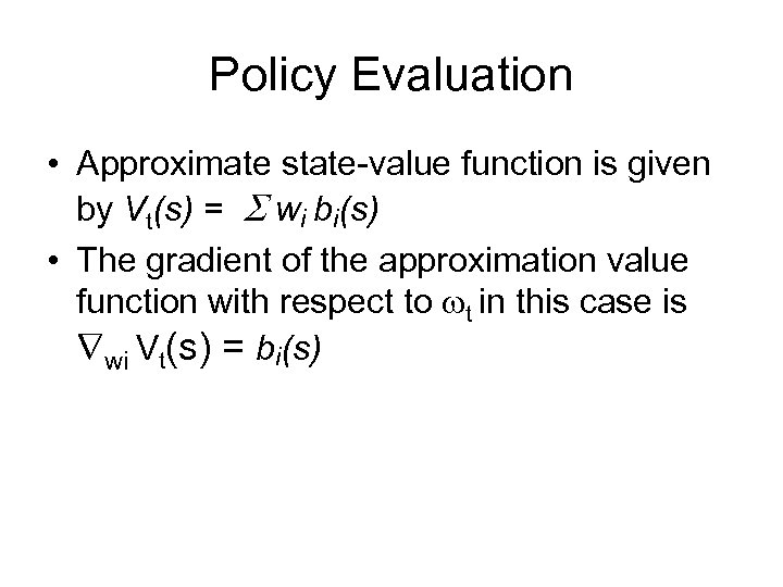Policy Evaluation • Approximate state-value function is given by Vt(s) = S wi bi(s) • The gradient of the approximation value function with respect to t in this case is wi Vt(s) = bi(s)

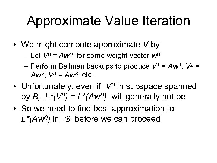Approximate Value Iteration • We might compute approximate V by – Let V 0 = Aw 0 for some weight vector w 0 – Perform Bellman backups to produce V 1 = Aw 1; V 2 = Aw 2; V 3 = Aw 3; etc. . . • Unfortunately, even if V 0 in subspace spanned by B, L*(V 0) = L*(Aw 0) will generally not be • So we need to find best approximation to L*(Aw 0) in B before we can proceed

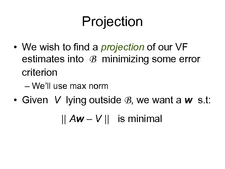Projection • We wish to find a projection of our VF estimates into B minimizing some error criterion – We’ll use max norm • Given V lying outside B, we want a w s. t: || Aw – V || is minimal

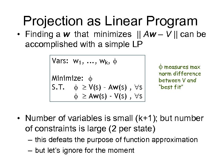Projection as Linear Program • Finding a w that minimizes || Aw – V || can be accomplished with a simple LP Vars: w 1, . . . , wk, f Minimize: f S. T. f V(s) – Aw(s) , s f Aw(s) - V(s) , s f measures max norm difference between V and “best fit” • Number of variables is small (k+1); but number of constraints is large (2 per state) – this defeats the purpose of function approximation – but let’s ignore for the moment

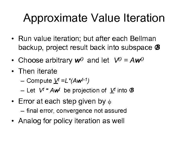Approximate Value Iteration • Run value iteration; but after each Bellman backup, project result back into subspace B • Choose arbitrary w 0 and let V 0 = Aw 0 • Then iterate – Compute Vt =L*(Awt-1) – Let Vt = Awt be projection of Vt into B • Error at each step given by f – final error, convergence not assured • Analog for policy iteration as well

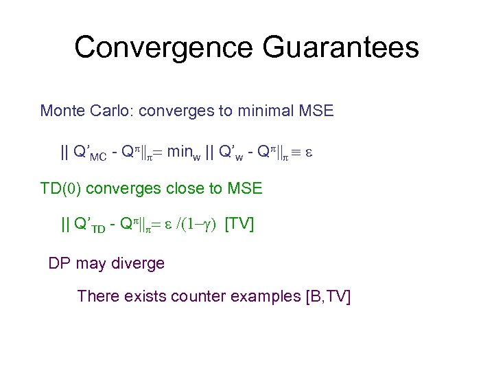Convergence Guarantees Monte Carlo: converges to minimal MSE || Q’MC - Q || = minw || Q’w - Q || º TD(0) converges close to MSE || Q’TD - Q || = /(1 - ) [TV] DP may diverge There exists counter examples [B, TV]

VFA Convergence results • Linear TD( ) converges if we visit states using the onpolicy distribution • Off policy Linear TD( ) and linear Q learning are known to diverge in some cases • Q-learning, and value iteration used with some averagers (including k-Nearest Neighbour and decision trees) has almost sure convergence if particular exploration policies are used • A special case of policy iteration with Sarsa style updates and linear function approximation converges • Residual algorithms are guaranteed to converge but only very slowly

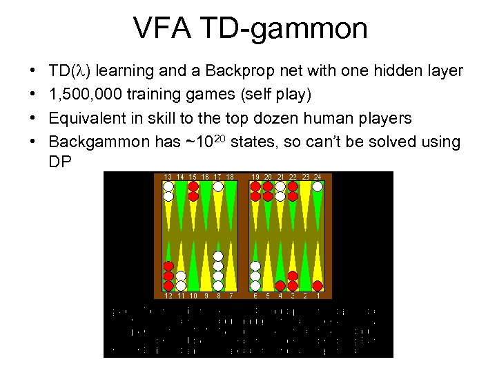VFA TD-gammon • • TD( ) learning and a Backprop net with one hidden layer 1, 500, 000 training games (self play) Equivalent in skill to the top dozen human players Backgammon has ~1020 states, so can’t be solved using DP

Homework • Read about POMDPs: [Littman ’ 96] Ch. 6 -7

• THE END

FA, is it the answer? • Not all FA methods are suited for the use of RL. For example, NN and statistical methods assume a static training set over which multiple passes are made. In RL, however, it is important that learning be able to ccur on-line, while interacting with the environment (or a model of the environment) • In particular, Q learning seems to lose its convergence properties when integrated with FA

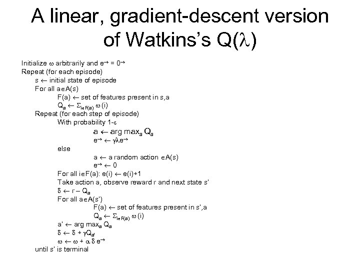A linear, gradient-descent version of Watkins’s Q( ) Initialize arbitrarily and e = 0 Repeat (for each episode) s initial state of episode For all a A(s) F(a) set of features present in s, a Qa i F(a) (i) Repeat (for each step of episode) With probability 1 - a arg maxa Qa e e else a a random action A(s) e 0 For all i F(a): e(i)+1 Take action a, observe reward r and next state s’ r – Qa For all a A(s’) F(a) set of features present in s’, a Qa i F(a) (i) a’ arg maxa Qa + Qa’ + e until s’ is terminal