Dealing with MASSIVE Data Feifei Li lifeifei cs fsu

Dealing with MASSIVE Data Feifei Li lifeifei@cs. fsu. edu Dept Computer Science, FSU Sep 9, 2008

Brief Bio • B. A. S. in computer engineering from Nanyang Technological University in 2002 • Ph. D. in computer science from Boston University in 2007 • Research Interns/Visitors at AT&T Labs, IBM T. J. Watson Research Center, Microsoft Research. • Now: Assistant Professor in CS Department at FSU 2

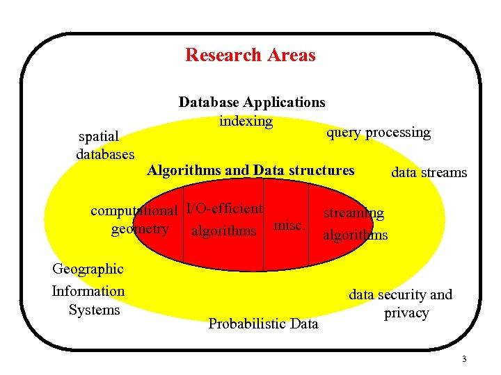Research Areas spatial databases Database Applications indexing Algorithms and Data structures computational I/O-efficient geometry algorithms misc. Geographic Information Systems query processing Probabilistic Data data streams streaming algorithms data security and privacy 3

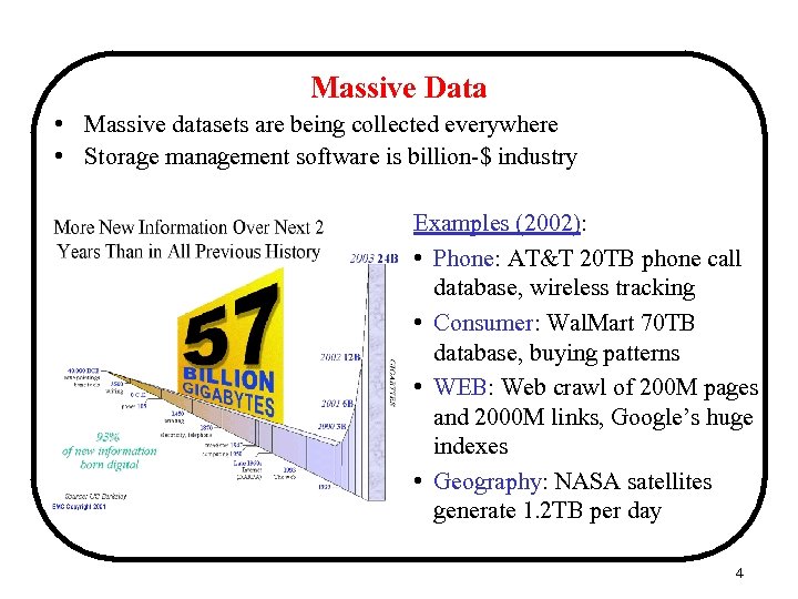Massive Data • Massive datasets are being collected everywhere • Storage management software is billion-$ industry Examples (2002): • Phone: AT&T 20 TB phone call database, wireless tracking • Consumer: Wal. Mart 70 TB database, buying patterns • WEB: Web crawl of 200 M pages and 2000 M links, Google’s huge indexes • Geography: NASA satellites generate 1. 2 TB per day 4

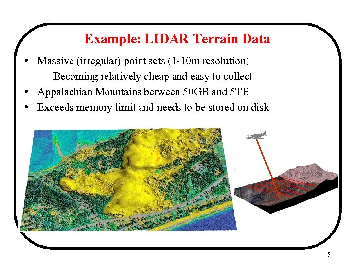Example: LIDAR Terrain Data • Massive (irregular) point sets (1 -10 m resolution) – Becoming relatively cheap and easy to collect • Appalachian Mountains between 50 GB and 5 TB • Exceeds memory limit and needs to be stored on disk 5

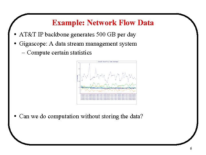Example: Network Flow Data • AT&T IP backbone generates 500 GB per day • Gigascope: A data stream management system – Compute certain statistics • Can we do computation without storing the data? 6

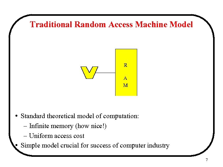Traditional Random Access Machine Model R A M • Standard theoretical model of computation: – Infinite memory (how nice!) – Uniform access cost • Simple model crucial for success of computer industry 7

How to Deal with MASSIVE Data? when there is not enough memory

Solution 1: Buy More Memory • Expensive • (Probably) not scalable – Growth rate of data is higher than the growth of memory 9

Solution 2: Cheat! (by random sampling) • Provide approximate solution for some problems – average, frequency of an element, etc. • What if we want the exact result? • Many problems can’t be solved by sampling – maximum, and all problems mentioned later 10

Solution 3: Using the Right Computation Model • External Memory Model • Streaming Model • Probabilistic Model (brief)

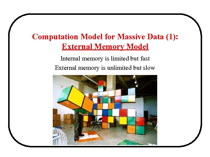Computation Model for Massive Data (1): External Memory Model Internal memory is limited but fast External memory is unlimited but slow

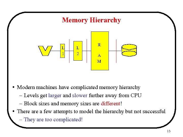Memory Hierarchy L 1 L 2 R A M • Modern machines have complicated memory hierarchy – Levels get larger and slower further away from CPU – Block sizes and memory sizes are different! • There a few attempts to model the hierarchy but not successful – They are too complicated! 13

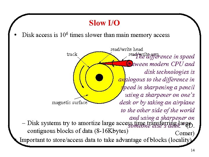Slow I/O • Disk access is 106 times slower than main memory access track read/write head read/write arm “The difference in speed between modern CPU and disk technologies is analogous to the difference in speed in sharpening a pencil using a sharpener on one’s magnetic surface desk or by taking an airplane to the other side of the world and using a sharpener on – Disk systems try to amortize large access time transferring large someone else’s desk. ” (D. contiguous blocks of data (8 -16 Kbytes) Comer) • Important to store/access data to take advantage of blocks (locality) 14

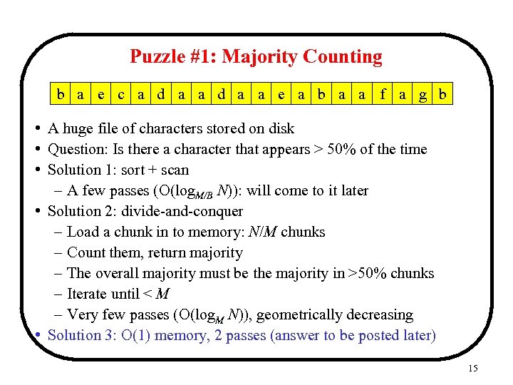Puzzle #1: Majority Counting b a e c a d a a e a b a a f a g b • A huge file of characters stored on disk • Question: Is there a character that appears > 50% of the time • Solution 1: sort + scan – A few passes (O(log. M/B N)): will come to it later • Solution 2: divide-and-conquer – Load a chunk in to memory: N/M chunks – Count them, return majority – The overall majority must be the majority in >50% chunks – Iterate until < M – Very few passes (O(log. M N)), geometrically decreasing • Solution 3: O(1) memory, 2 passes (answer to be posted later) 15

External Memory Model [AV 88] D Block I/O M N = # of items in the problem instance B = # of items per disk block M = # of items that fit in main memory I/O: Move block between memory and disk Performance measure: # of I/Os performed by algorithm P We assume (for convenience) that M >B 2 16

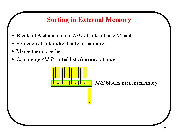Sorting in External Memory • • Break all N elements into N/M chunks of size M each Sort each chunk individually in memory Merge them together Can merge

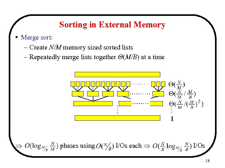Sorting in External Memory • Merge sort: – Create N/M memory sized sorted lists – Repeatedly merge lists together Θ(M/B) at a time phases using I/Os each I/Os 18

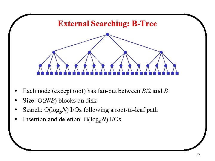External Searching: B-Tree • • Each node (except root) has fan-out between B/2 and B Size: O(N/B) blocks on disk Search: O(log. BN) I/Os following a root-to-leaf path Insertion and deletion: O(log. BN) I/Os 19

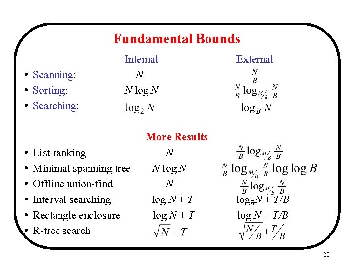Fundamental Bounds • Scanning: • Sorting: • Searching: • • • Internal N N log N List ranking Minimal spanning tree Offline union-find Interval searching Rectangle enclosure R-tree search More Results N N log N + T External log. BN + T/B log N + T/B 20

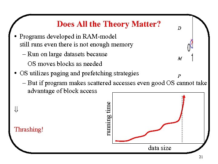Does All the Theory Matter? D Thrashing! running time • Programs developed in RAM-model still runs even there is not enough memory – Run on large datasets because M OS moves blocks as needed • OS utilizes paging and prefetching strategies P – But if program makes scattered accesses even good OS cannot take advantage of block access data size 21

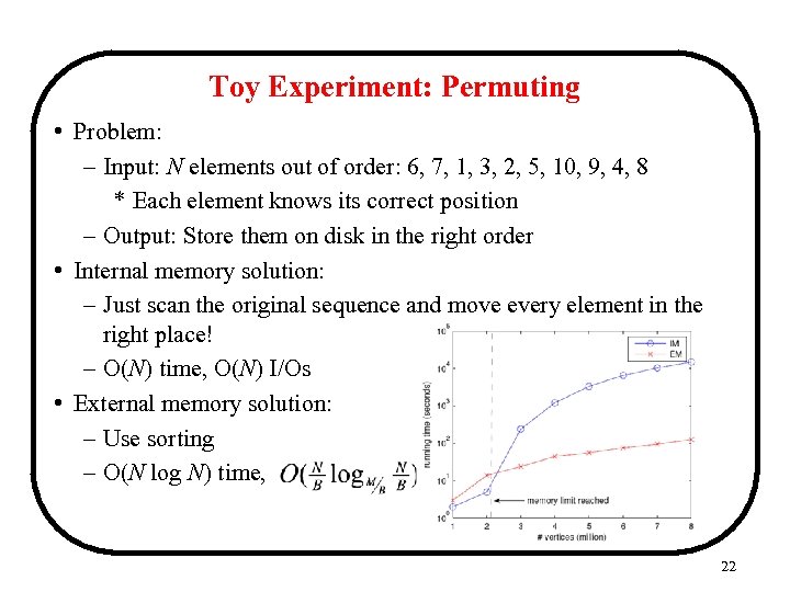Toy Experiment: Permuting • Problem: – Input: N elements out of order: 6, 7, 1, 3, 2, 5, 10, 9, 4, 8 * Each element knows its correct position – Output: Store them on disk in the right order • Internal memory solution: – Just scan the original sequence and move every element in the right place! – O(N) time, O(N) I/Os • External memory solution: – Use sorting – O(N log N) time, I/Os 22

A Practical Example on Real Data • Computing persistence on large terrain data 23

Takeaways • Need to be very careful when your program’s space usage exceeds physical memory size • If program mostly makes highly localized accesses – Let the OS handle it automatically • If program makes many non-localized accesses – Need I/O-efficient techniques • Three common techniques (recall the majority counting puzzle): – Convert to sort + scan – Divide-and-conquer – Other tricks 24

Want to know more about I/O-efficient algorithms? A course on I/O-efficient algorithms is offered as CIS 5930 (Advanced Topics in Data Management)

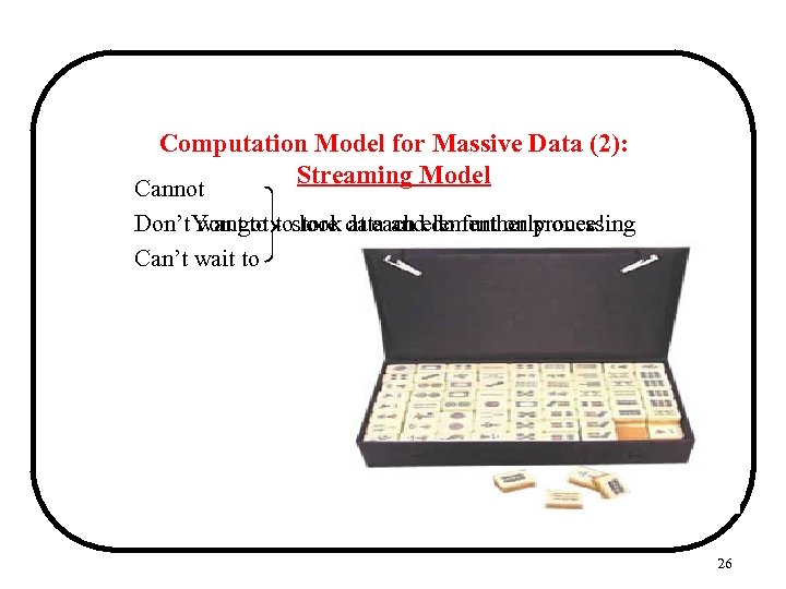Computation Model for Massive Data (2): Streaming Model Cannot Don’t. You got tostore data andelement only once! want to look at each do further processing Can’t wait to 26

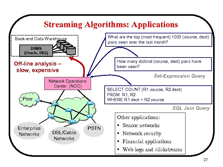Streaming Algorithms: Applications What are the top (most frequent) 1000 (source, dest) pairs seen over the last month? Back-end Data Warehouse DBMS (Oracle, DB 2) How many distinct (source, dest) pairs have been seen? Off-line analysis – slow, expensive Set-Expression Query Network Operations Center (NOC) SELECT COUNT (R 1. source, R 2. dest) FROM R 1, R 2 WHERE R 1. dest = R 2. source Peer SQL Join Query Enterprise Networks DSL/Cable Networks PSTN Other applications: • Sensor networks • Network security • Financial applications • Web logs and clickstreams 27

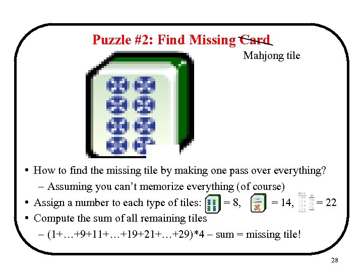Puzzle #2: Find Missing Card Mahjong tile • How to find the missing tile by making one pass over everything? – Assuming you can’t memorize everything (of course) • Assign a number to each type of tiles: = 8, = 14, = 22 • Compute the sum of all remaining tiles – (1+…+9+11+…+19+21+…+29)*4 – sum = missing tile! 28

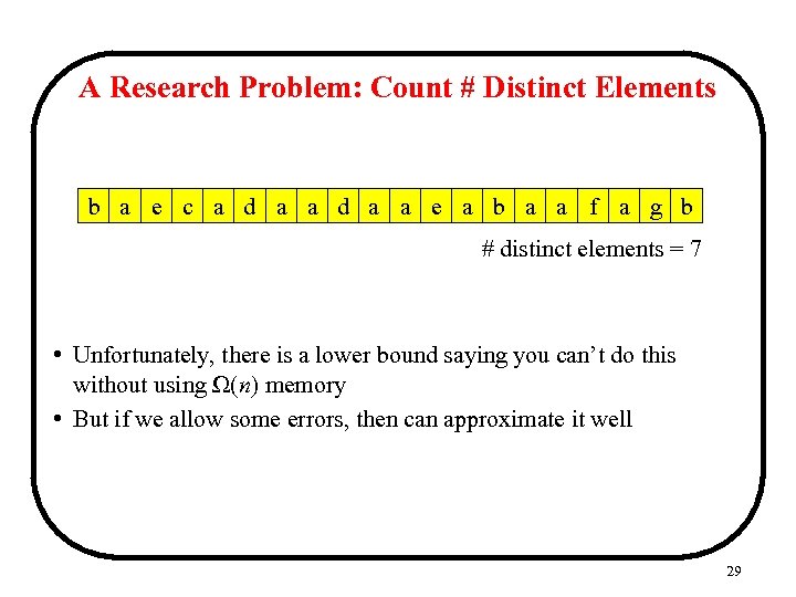A Research Problem: Count # Distinct Elements b a e c a d a a e a b a a f a g b # distinct elements = 7 • Unfortunately, there is a lower bound saying you can’t do this without using Ω(n) memory • But if we allow some errors, then can approximate it well 29

Solution: FM Sketch [FM 85, AMS 99] • Take a (pseudo) random hash function h : {1, …, n} {1, …, 2 d}, where 2 d > n • For each incoming element x, compute h(x) – e. g. , h(5) = 1010110000 – Count how many trailing zeros – Remember the maximum number of trailing zeroes in any h(x) • Let Y be the maximum number of trailing zeroes – Can show E[2 Y] = # distinct elements * 2 elements, “on average” there is one h(x) with 1 trailing zero * 4 elements, “on average” there is one h(x) with 2 trailing zeroes * 8 elements, “on average” there is one h(x) with 3 trailing zeroes *… 30

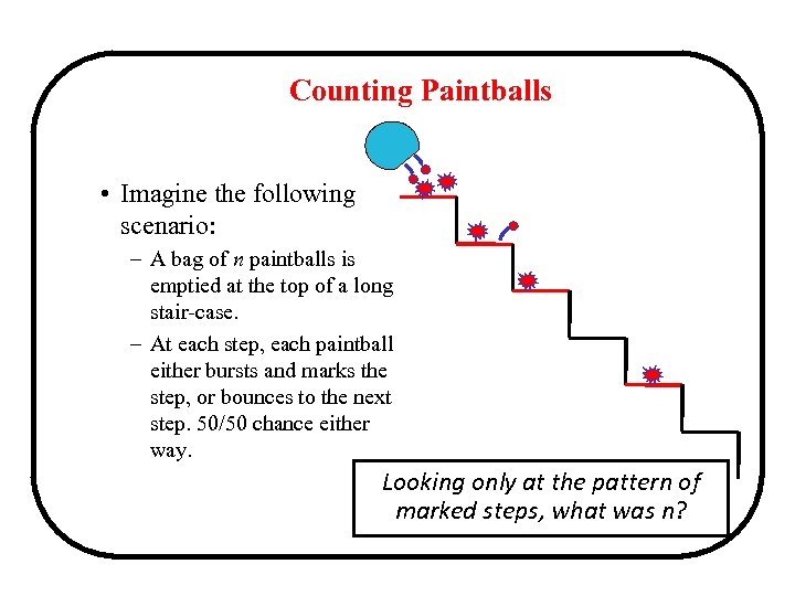Counting Paintballs • Imagine the following scenario: – A bag of n paintballs is emptied at the top of a long stair-case. – At each step, each paintball either bursts and marks the step, or bounces to the next step. 50/50 chance either way. Looking only at the pattern of marked steps, what was n?

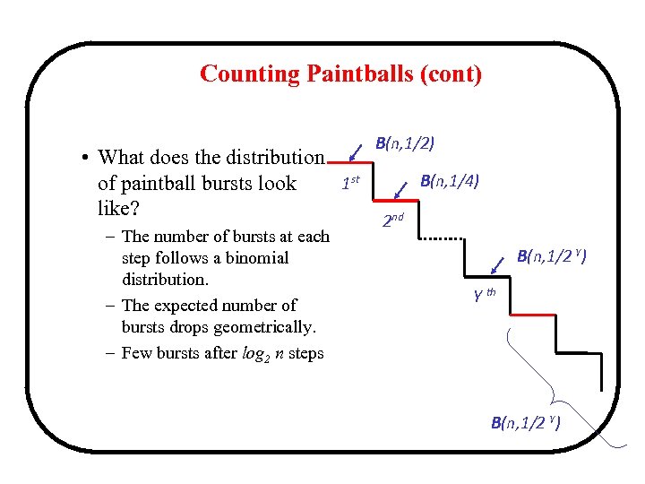Counting Paintballs (cont) • What does the distribution 1 st of paintball bursts look like? – The number of bursts at each step follows a binomial distribution. – The expected number of bursts drops geometrically. – Few bursts after log 2 n steps B(n, 1/2) B(n, 1/4) 2 nd B(n, 1/2 Y) Y th B(n, 1/2 Y)

Solution: FM Sketch [FM 85, AMS 99] • So 2 Y is an unbiased estimator for # distinct elements • However, has a large variance – Use O(1/ε 2 ∙ log(1/δ)) copies to guarantee a good estimator that has probability 1–δ to be within relative error ε • Applications: – How many distinct IP addresses used a given link to send their traffic from the beginning of the day? – How many new IP addresses appeared today that didn’t appear before? 33

Finding Heavy Hitters • Which elements appeared in the stream more than 10% of the time? • Applications: – Networking * Finding IP addresses sending most traffic – Databases * Iceberg queries – Data mining * Finding “hot” items (item sets) in transaction data • Solution – Exact solution is difficult – If allow approximation of ε * Use O(1/ε) space and O(1) time per element in stream 34

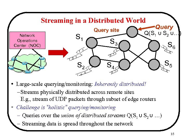Streaming in a Distributed World Network Operations Center (NOC) Query site S 1 S 3 1 1 0 Q(S 1 ∪ S 2 ∪…) 1 1 S 2 0 1 0 S 6 1 1 0 Query S 4 0 1 1 1 0 S 5 1 0 • Large-scale querying/monitoring: Inherently distributed! – Streams physically distributed across remote sites E. g. , stream of UDP packets through subset of edge routers • Challenge is “holistic” querying/monitoring – Queries over the union of distributed streams Q(S 1 ∪ S 2 ∪ …) – Streaming data is spread throughout the network 35

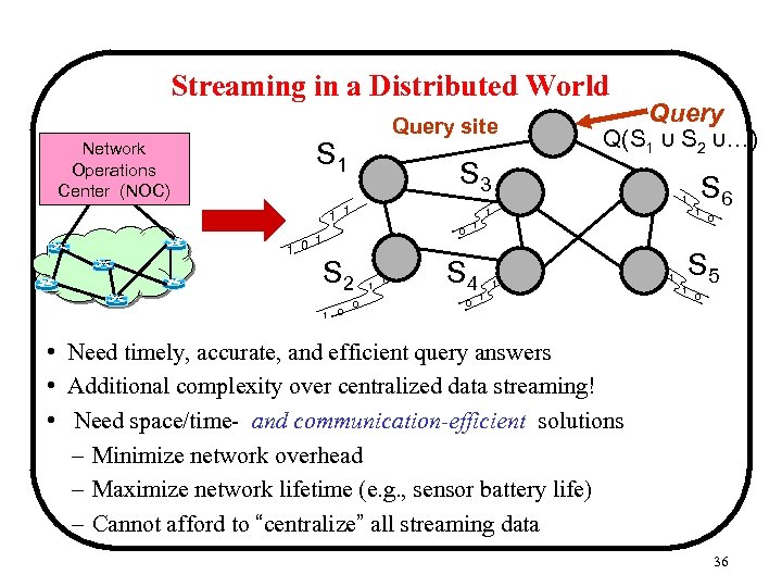Streaming in a Distributed World Network Operations Center (NOC) Query site S 1 S 3 1 1 0 Q(S 1 ∪ S 2 ∪…) 1 1 S 2 0 1 0 S 6 1 1 0 Query S 4 0 1 1 1 0 S 5 1 0 • Need timely, accurate, and efficient query answers • Additional complexity over centralized data streaming! • Need space/time- and communication-efficient solutions – Minimize network overhead – Maximize network lifetime (e. g. , sensor battery life) – Cannot afford to “centralize” all streaming data 36

Want to know more about streaming algorithms? A graduate-level course on streaming algorithms will be approximately offered in the next semester with an error guarantee of 5%! Or, talk to me tomorrow!

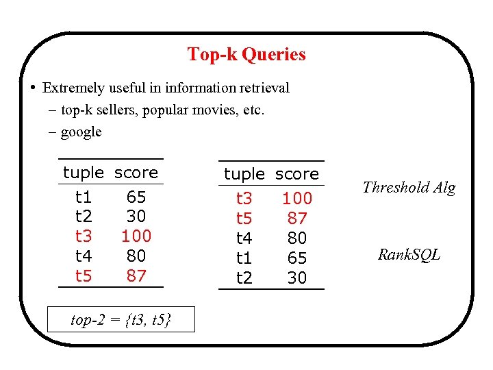Top-k Queries • Extremely useful in information retrieval – top-k sellers, popular movies, etc. – google tuple score t 1 65 t 2 30 t 3 100 t 4 80 t 5 87 top-2 = {t 3, t 5} tuple score t 3 100 t 5 87 t 4 80 t 1 65 t 2 30 Threshold Alg Rank. SQL

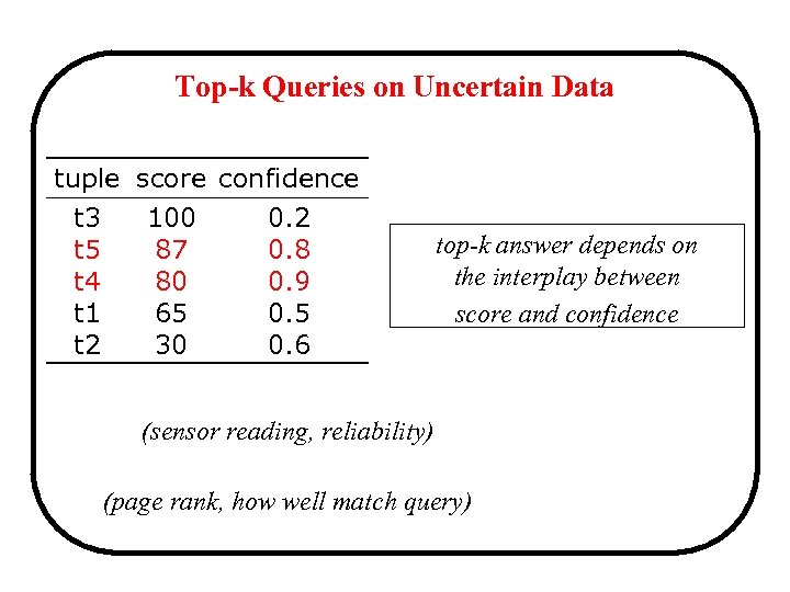Top-k Queries on Uncertain Data tuple score confidence t 3 100 0. 2 t 5 87 0. 8 t 4 80 0. 9 t 1 65 0. 5 t 2 30 0. 6 top-k answer depends on the interplay between score and confidence (sensor reading, reliability) (page rank, how well match query)

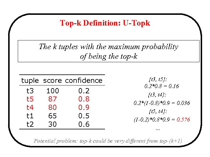Top-k Definition: U-Topk The k tuples with the maximum probability of being the top-k tuple score confidence t 3 100 0. 2 t 5 87 0. 8 t 4 80 0. 9 t 1 65 0. 5 t 2 30 0. 6 {t 3, t 5}: 0. 2*0. 8 = 0. 16 {t 3, t 4}: 0. 2*(1 -0. 8)*0. 9 = 0. 036 {t 5, t 4}: (1 -0. 2)*0. 8*0. 9 = 0. 576. . . Potential problem: top-k could be very different from top-(k+1)

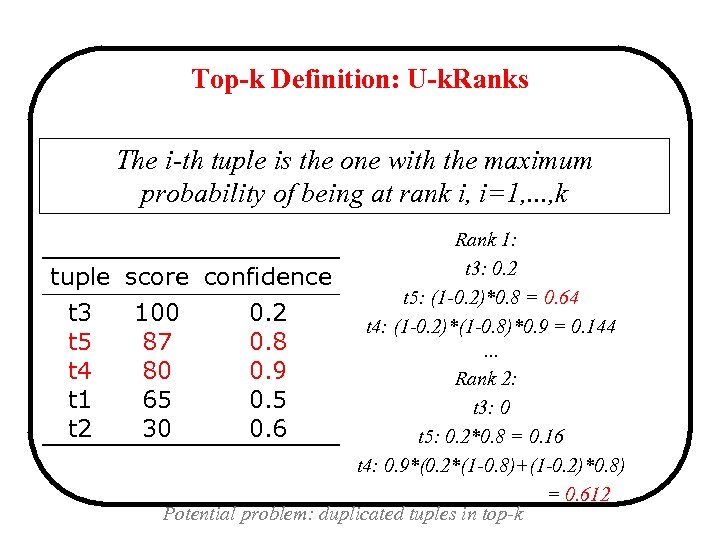Top-k Definition: U-k. Ranks The i-th tuple is the one with the maximum probability of being at rank i, i=1, . . . , k tuple t 3 t 5 t 4 t 1 t 2 Rank 1: t 3: 0. 2 score confidence t 5: (1 -0. 2)*0. 8 = 0. 64 100 0. 2 t 4: (1 -0. 2)*(1 -0. 8)*0. 9 = 0. 144 87 0. 8. . . 80 0. 9 Rank 2: 65 0. 5 t 3: 0 30 0. 6 t 5: 0. 2*0. 8 = 0. 16 t 4: 0. 9*(0. 2*(1 -0. 8)+(1 -0. 2)*0. 8) = 0. 612 Potential problem: duplicated tuples in top-k

Uncertain Data Models • An uncertain data model represents a probability distribution of database instances (possible worlds) • Basic model: mutual independence among all tuples • Complete models: able to represent any distribution of possible worlds – Atomic independent random Boolean variables – Each tuple corresponds to a Boolean formula, appears iff the formula evaluates to true – Exponential complexity

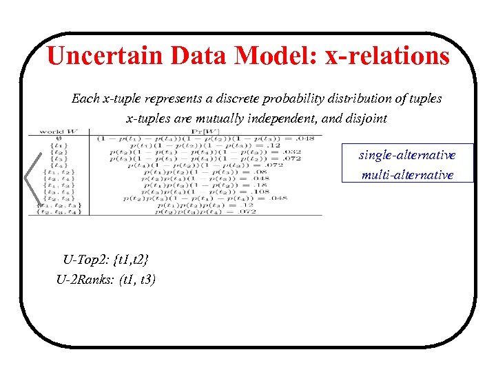Uncertain Data Model: x-relations Each x-tuple represents a discrete probability distribution of tuples x-tuples are mutually independent, and disjoint single-alternative multi-alternative U-Top 2: {t 1, t 2} U-2 Ranks: (t 1, t 3)

Want to know more about uncertainty data management? A graduate-level course on uncertainty data management will be (likely probably) offered in the next next semester Or, talk to me tomorrow!

Recap • External memory model – Main memory is fast but limited – External memory slow but unlimited – Aim to optimize I/O performance • Streaming model – Main memory is fast but small – Can’t store, not willing to store, or can’t wait to store data – Compute the desired answers in one pass • Probabilistic data model – Can’t store, query exponential possible instances of possible worlds – Compute the desired answers in the succinct representation of the probabilistic data (efficiently!! Possibly allow some errors) 45

Thanks! Questions?