10293420997c01f00f6142a677539b01.ppt
- Количество слайдов: 138

+ Databases and Information Retrieval Integration TIETS 42 Preferences in Databases Autumn 2016 Kostas Stefanidis kostas. stefanidis@uta. fi http: //www. uta. fi/sis/tie/dbir/index. html http: //people. uta. fi/~kostas. stefanidis/dbir 16 -main. html

Introduction Preferences guide human decisions e. g. , “which ice-cream flavor to buy? ” e. g. , “which investment funds to choose? ” Preferences have been studied in philosophy, psychology, economics, etc e. g. , in philosophy: reasoning on values, desires, duties TODAY’s topic Preferences in Databases : 2
Introduction Why considering preferences in databases? What are the challenges? What has been done so far? What next? 3
Why Preferences in Databases? The Boolean database answer model: all or nothing! Empty-answer problem Too-many-answers problem Databases on the Web: 7, 500 TB (19 TB is the surface Web)! • National Climatic Data Center (NOAA) • NASA EOSDIS • Alexandria Digital Library • JSTOR Project Limited • US Census • Amazon. com • … 4
Why Preferences in Databases? The Boolean database answer model: all or nothing! Empty-answer problem Too-many-answers problem Databases on the Web: 7, 500 TB (19 TB is the surface Web!) Unknown schema Unknown contents On the Web: Too much information Information Overload User diversity 5
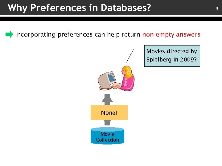
Why Preferences in Databases? Incorporating preferences can help return non-empty answers Movies directed by Spielberg in 2009? None! Movie Collection 6

Why Preferences in Databases? 7 Incorporating preferences can help return non-empty answers Movies directed by Spielberg in 2009? I like adventures I like Spielberg A 2008 Spielberg movie Inglourious Basterds Star Trek Indiana Jones Movie Collection

Why Preferences in Databases? Incorporating preferences can help return focused answers movies K-19 Analyze this Bananas Movie Collection 8

Why Preferences in Databases? 9 Incorporating preferences can help return focused answers comedymovies not by W. Allen movies adventure K-19 Bananas W. Allen movie W. Allen adventure Analyze this Movie Collection comedy not W. Allen

Tutorial Overview Preference Representation Preference Composition Preferential Query Processing 10
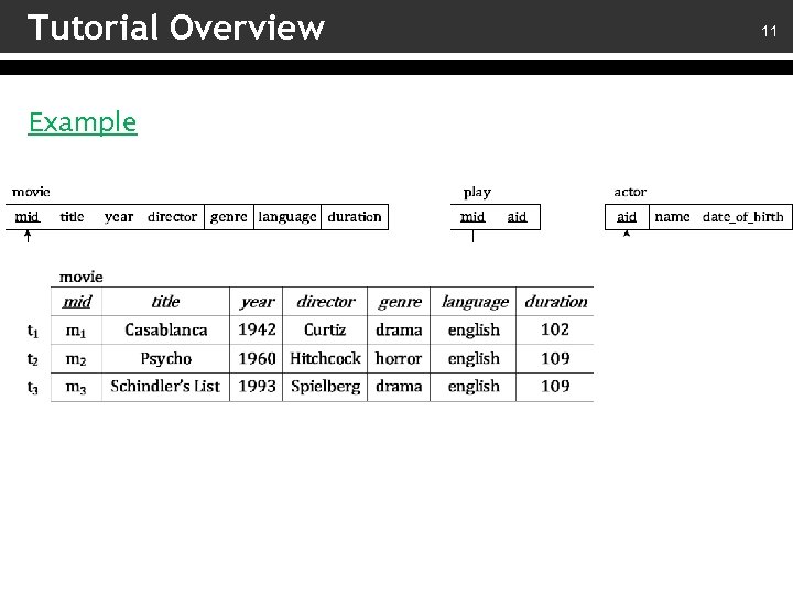
Tutorial Overview Example 11
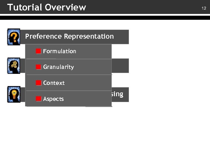
Tutorial Overview Preference Representation Formulation Preference Composition Granularity Context Preferential Query Processing Aspects Preference Learning 12
Formulation Qualitative approaches Quantitative approaches 13

Formulation: Qualitative Approaches Binary preference relations Preferences between tuples in the answer to a query are specified directly using binary preference relations [Chomicki 2003; Kiessling 2002] Given a relation R: A preference relation B is a subset of R×R a B b between tuples a and b of R => a is preferred over b 14

Formulation: Qualitative Approaches Logical formulas A logical formula PF expresses the constraints two tuples must satisfy so that one is preferred over the other [Chomicki 2003; Georgiadis et al. 2008] ti ≻PF tj ti[genre] = tj[genre] ti[duration] < tj[duration] Casablanca is preferred over Schindler’s list 15

Formulation: Qualitative Approaches Preference Constructors A formal language formulating preference relations using constructors [Kiessling 2002] HIGHEST(A) {ti ≻ P_new tj iff ti > tj}; AROUND(A, z) {ti ≻ P_new tj iff abs(ti z) < abs(tj z)}; 16

Formulation: Qualitative Approaches Preference Constructors A formal language formulating preference relations using constructors [Kiessling 2002] POS(genre, {horror}) NEG(year, {1960}) EXP(title, {(Casablanca), (Psycho), (Schindler’s list)}) 17
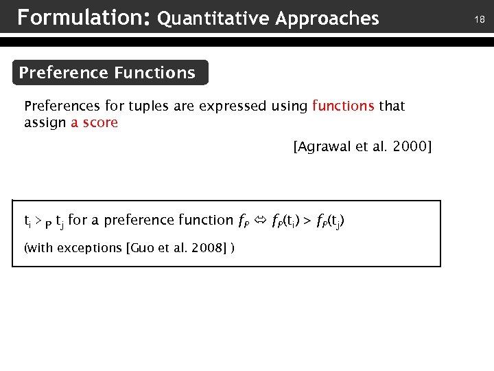
Formulation: Quantitative Approaches Preference Functions Preferences for tuples are expressed using functions that assign a score [Agrawal et al. 2000] ti ≻ P tj for a preference function f. P(ti) > f. P(tj) (with exceptions [Guo et al. 2008] ) 18

Formulation: Quantitative Approaches 19 Preference Functions Example 0. 102 0. 109 f. P(ti) = 0. 001 × ti[duration]
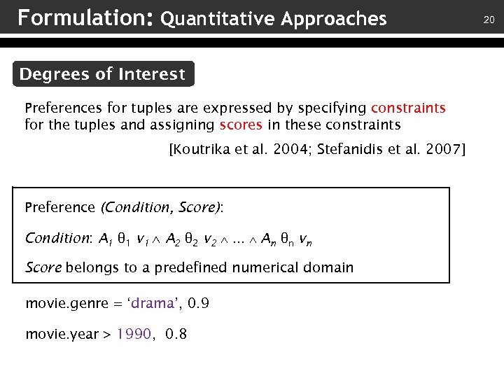
Formulation: Quantitative Approaches Degrees of Interest Preferences for tuples are expressed by specifying constraints for the tuples and assigning scores in these constraints [Koutrika et al. 2004; Stefanidis et al. 2007] Preference (Condition, Score): Condition: A 1 θ 1 v 1 A 2 θ 2 v 2 … An θn vn Score belongs to a predefined numerical domain movie. genre = ‘drama’, 0. 9 movie. year > 1990, 0. 8 20
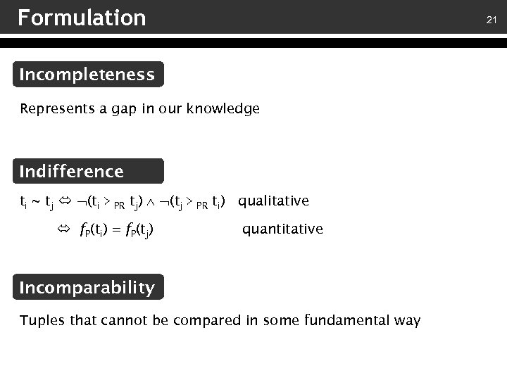
Formulation 21 Incompleteness Represents a gap in our knowledge Indifference ti ~ tj (ti ≻ PR tj) (tj ≻ PR ti) qualitative f. P(ti) = f. P(tj) quantitative Incomparability Tuples that cannot be compared in some fundamental way
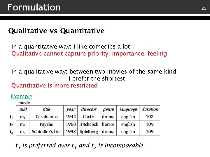
Formulation Qualitative vs Quantitative In a quantitative way: I like comedies a lot! Qualitative cannot capture priority, importance, feeling In a qualitative way: between two movies of the same kind, I prefer the shortest Quantitative is more restricted Example t 3 is preferred over t 1 and t 2 is incomparable 22
Preference Representation Preference representation dimensions Formulation Granularity Context Aspects 23

Granularity 24 Tuple Preferences expressed directly for tuples and their values movie. genre = ‘drama’, movie. mid = cast. mid and cast. aid = actor. aid and actor. name = ‘J. Roberts’, 0. 9 0. 7 [Koutrika and Ioannidis 2010]
Granularity 25 Set Preferences expressed based on the properties of a group of tuples as a whole [Zhang and Chomicki 2008] I want to see three movies of the same director
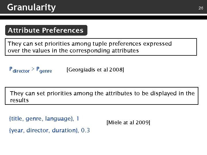
Granularity 26 Attribute Preferences They can set priorities among tuple preferences expressed over the values in the corresponding attributes Pdirector ≻ Pgenre [Georgiadis et al 2008] They can set priorities among the attributes to be displayed in the results {title, genre, language}, 1 {year, director, duration}, 0. 3 [Miele at al 2009]

Granularity 27 Relationship Preferences They are expressed on relationships between two types of entities or two particular entities (movie. mid = play. mid, 1) [Koutrika, Ioannidis 2004] A director has directed many movies Julia Roberts has acted in Ocean’s Eleven
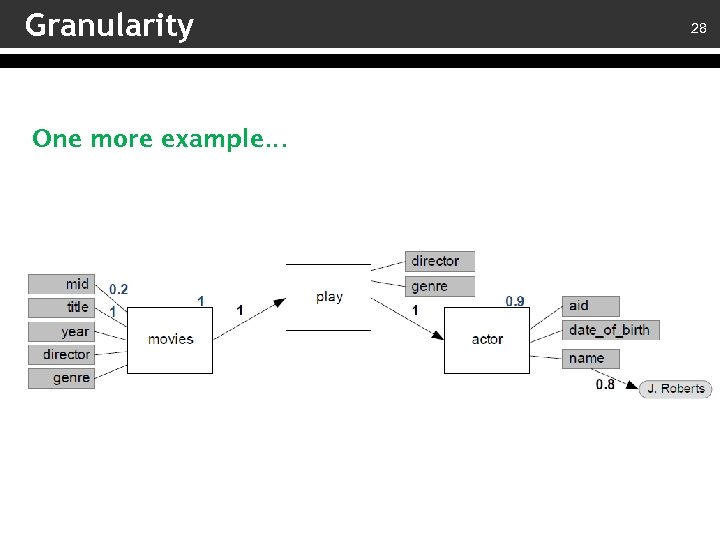
Granularity One more example… 28

Preference Representation Preference representation dimensions Formulation Granularity Context Aspects 29
Context 30 Context is any information that can be used to characterize the situation of an entity An entity is a person, place, object that is considered relevant to the interaction between a user and an application, including the user and the application themselves [Dey 2001] User preferences can be part of the user context! We study how context determined when user preferences hold
Context (in preferences) Context is any external to the database information that can be used to characterize the situation of a user or any internally stored information that can be used to characterize the data per se 31
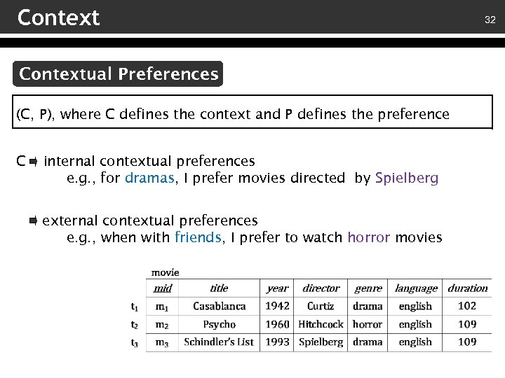
Contextual Preferences (C, P), where C defines the context and P defines the preference C internal contextual preferences e. g. , for dramas, I prefer movies directed by Spielberg external contextual preferences e. g. , when with friends, I prefer to watch horror movies 32
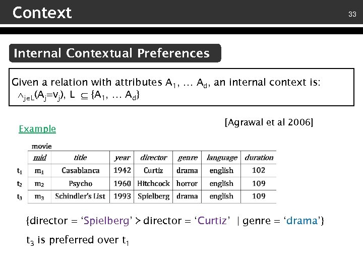
Context 33 Internal Contextual Preferences Given a relation with attributes A 1, … Ad, an internal context is: j L(Aj=vj), L {A 1, … Ad} Example [Agrawal et al 2006] {director = ‘Spielberg’ ≻ director = ‘Curtiz’ | genre = ‘drama’} t 3 is preferred over t 1
![Context 34 Internal Contextual Preferences Example ti ≻ PF tj [Chomicki 2003] (ti[genre] = Context 34 Internal Contextual Preferences Example ti ≻ PF tj [Chomicki 2003] (ti[genre] =](https://present5.com/presentation/10293420997c01f00f6142a677539b01/image-34.jpg)
Context 34 Internal Contextual Preferences Example ti ≻ PF tj [Chomicki 2003] (ti[genre] = tj[genre] ti[genre] = ‘drama’ ti[director] = ‘Spielberg’ tj[director] = ‘Curtiz’ ) (ti[genre] = tj[genre] ti[genre] = ‘thriller’ tj[director] = ‘Spielberg’ ti[director] = ‘Curtiz’ )
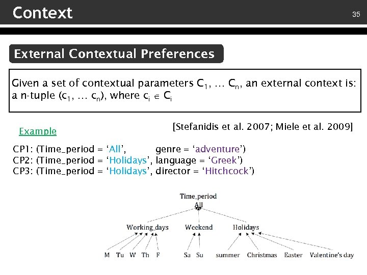
Context 35 External Contextual Preferences Given a set of contextual parameters C 1, … Cn, an external context is: a n-tuple (c 1, … cn), where ci Ci Example [Stefanidis et al. 2007; Miele et al. 2009] CP 1: (Time_period = ‘All’, genre = ‘adventure’) CP 2: (Time_period = ‘Holidays’, language = ‘Greek’) CP 3: (Time_period = ‘Holidays’, director = ‘Hitchcock’)
Preference Representation Preference representation dimensions Formulation Granularity Context Aspects 36
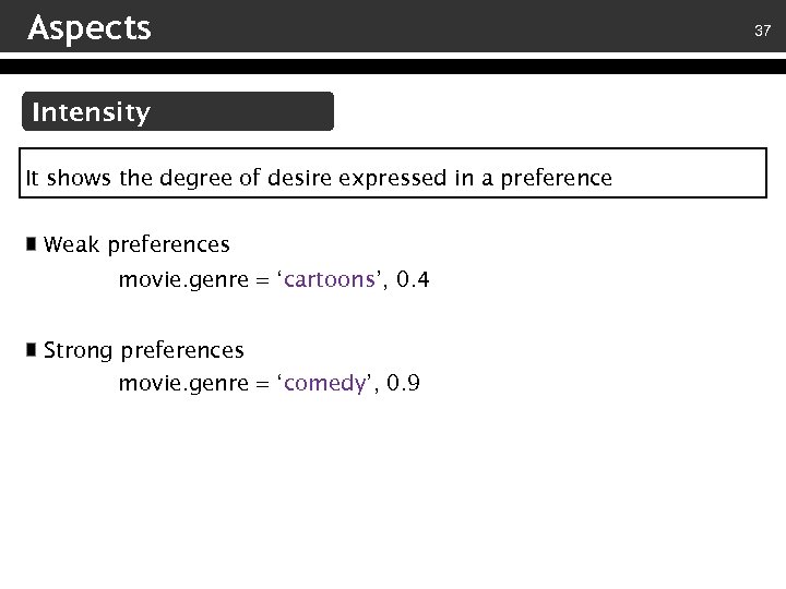
Aspects Intensity It shows the degree of desire expressed in a preference Weak preferences movie. genre = ‘cartoons’, 0. 4 Strong preferences movie. genre = ‘comedy’, 0. 9 37
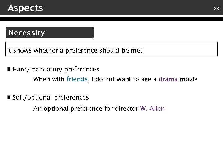
Aspects Necessity It shows whether a preference should be met Hard/mandatory preferences When with friends, I do not want to see a drama movie Soft/optional preferences An optional preference for director W. Allen 38

Aspects Feeling It shows how one feels about something Positive preferences movie. genre = ‘drama’, 0. 9 Negative preferences movie. genre = ‘horror’, -0. 5 39
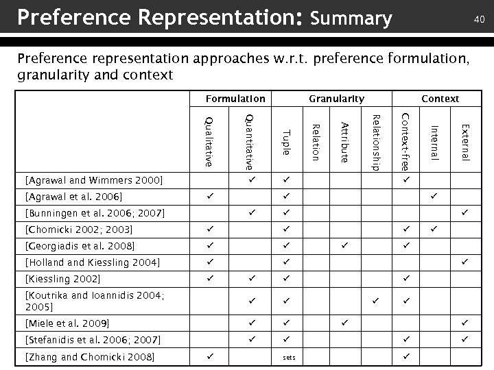
Preference Representation: Summary 40 Preference representation approaches w. r. t. preference formulation, granularity and context Formulation [Chomicki 2002; 2003] [Holland Kiessling 2004] [Kiessling 2002] [Georgiadis et al. 2008] [Koutrika and Ioannidis 2004; 2005] [Miele et al. 2009] [Stefanidis et al. 2006; 2007] sets [Zhang and Chomicki 2008] External Internal Context-free Relationship Attribute Tuple [Bunningen et al. 2006; 2007] Context Relation Quantitative Qualitative [Agrawal and Wimmers 2000] [Agrawal et al. 2006] Granularity
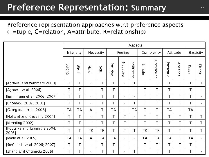
Preference Representation: Summary 41 Preference representation approaches w. r. t preference aspects (T=tuple, C=relation, A=attribute, R=relationship) Aspects Intensity Necessity Feeling Complexity Attitude Elasticity Strong Weak Hard Soft Positive Negative Indifferent Simple Compound Presence Absence Exact Elastic [Agrawal and Wimmers 2000] T T - T T T T [Agrawal et al. 2006] T T - - T T T - [Bunningen et al. 2006; 2007] T T - - T T T - [Chomicki 2002; 2003] T T - T T T - [Georgiadis et al. 2008] TA TA A T TA - TA T T TA - [Holland Kiessling 2004] T T - T T T T [Kiessling 2002] T T - T T T T [Koutrika and Ioannidis 2004; 2005] T T TR TR T T TA TA TA - - TA TA TA T TA - [Stefanidis et al. 2006; 2007] T T - - T T T [Zhang and Chomicki 2008] T T - T T T [Miele et al. 2009] -

Tutorial Overview Preference Representation Preference Composition Qualitative Composition Preferential Query Processing Quantitative Composition Heterogeneous Composition Preference Learning 42

Qualitative Composition mechanisms defined over preference relations – Prioritized Composition o E. g. , Px is considered more important than Py – Pareto Composition o Equally important preference relations – Pair-wise Comparisons Composition – Set-oriented Composition o Intersection, Union, Difference In following, we assume composition of two preferences Px and Py; generalizing to n > 2 preferences is straightforward 43
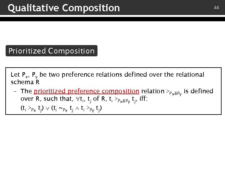
Qualitative Composition Prioritized Composition Let Px, Py be two preference relations defined over the relational schema R – The prioritized preference composition relation ≻Px&Py is defined over R, such that, ti, tj of R, ti ≻Px&Py tj, iff: (ti ≻Px tj) (ti ~Px tj ti ≻Py tj) 44
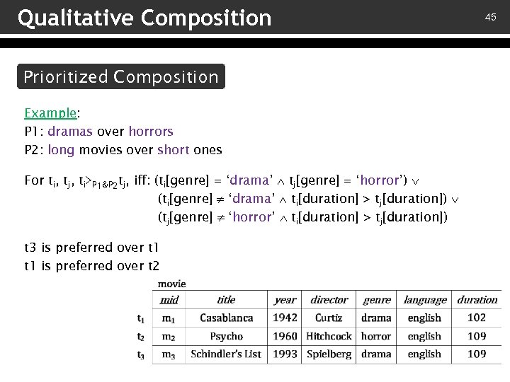
Qualitative Composition Prioritized Composition Example: P 1: dramas over horrors P 2: long movies over short ones For ti, tj, ti≻P 1&P 2 tj, iff: (ti[genre] = ‘drama’ tj[genre] = ‘horror’) (ti[genre] ‘drama’ ti[duration] > tj[duration]) (tj[genre] ‘horror’ ti[duration] > tj[duration]) t 3 is preferred over t 1 is preferred over t 2 45

Qualitative Composition 46 Prioritized composition over different relational schemas Lexicographical Composition For Px, Py defined over R, R’ with attribute domains dom(A), dom(A’) – The lexicographical preference composition relation ≻Px&Py defined over R×R’, is a subset of dom(A)×dom(A’), such that, (ti, t’i) ≻Px&Py (tj, t’j), iff: (ti ≻Px tj) (ti ~Px tj t’i ≻Py t’j) ti, tj are tuples of R and t’i, t’j tuples of R’
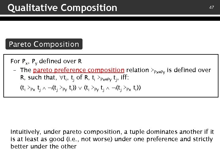
Qualitative Composition 47 Pareto Composition For Px, Py defined over R – The pareto preference composition relation ≻Px⊗Py is defined over R, such that, ti, tj of R, ti ≻Px⊗Py tj, iff: (ti ≻Px tj (tj ≻Py ti)) (ti ≻Py tj (tj ≻Px ti)) Intuitively, under pareto composition, a tuple dominates another if it is at least as good (i. e. , not worse) under one preference and strictly better under the other
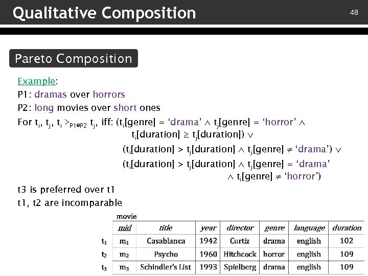
Qualitative Composition Pareto Composition Example: P 1: dramas over horrors P 2: long movies over short ones For ti, tj, ti ≻P 1⊗P 2 tj, iff: (ti[genre] = ‘drama’ tj[genre] = ‘horror’ ti[duration] ≥ tj[duration]) (ti[duration] > tj[duration] tj[genre] ‘drama’) (ti[duration] > tj[duration] tj[genre] = ‘drama’ ti[genre] ‘horror’) t 3 is preferred over t 1, t 2 are incomparable 48
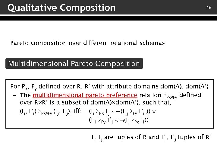
Qualitative Composition 49 Pareto composition over different relational schemas Multidimensional Pareto Composition For Px, Py defined over R, R’ with attribute domains dom(A), dom(A’) – The multidimensional pareto preference relation ≻Px⊗Py defined over R×R’ is a subset of dom(A)×dom(A’), such that, (ti, t’i) ≻Px⊗Py (tj, t’j), iff: (ti ≻Px tj (t’j ≻Py t’i )) (t’i ≻Py t’j (tj ≻Px ti)) ti, tj are tuples of R and t’i, t’j tuples of R’
![Qualitative Composition 50 Motivation: Voting theory [Condorcet 1785] Pair-wise Comparisons Composition Given a set Qualitative Composition 50 Motivation: Voting theory [Condorcet 1785] Pair-wise Comparisons Composition Given a set](https://present5.com/presentation/10293420997c01f00f6142a677539b01/image-50.jpg)
Qualitative Composition 50 Motivation: Voting theory [Condorcet 1785] Pair-wise Comparisons Composition Given a set of preference relations: ti is preferred over tj, iff, ti is preferred over tj for the majority of the preference relations Other methods of voting theory: – Given a set of rankings, tuples are ordered based on the number of times each one appears first – [Borda 1781]: determine the position of a tuple by the sum of its positions in the initial rankings
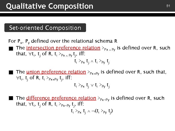
Qualitative Composition 51 Set-oriented Composition For Px, Py defined over the relational schema R – The intersection preference relation ≻Px Py is defined over R, such that, ti, tj of R, ti ≻Px Py tj, iff: ti ≻Px tj ti ≻Py tj – The union preference relation ≻Px+Py is defined over R, such that, ti, tj of R, ti ≻Px+Py tj, iff: ti ≻Px tj ti ≻Py tj – The difference preference relation ≻Px−Py is defined over R, such that, ti, tj of R, ti ≻Px−Py tj, iff: ti ≻Px tj (ti ≻Py tj)
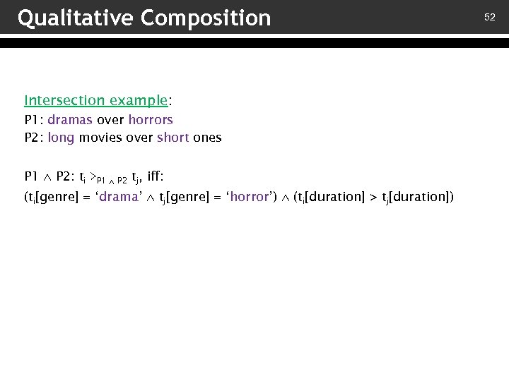
Qualitative Composition Intersection example: P 1: dramas over horrors P 2: long movies over short ones P 1 P 2: ti ≻P 1 P 2 tj, iff: (ti[genre] = ‘drama’ tj[genre] = ‘horror’) (ti[duration] > tj[duration]) 52
Preference Composition 53 Preference composition mechanism categories: – Qualitative composition – Quantitative composition o Combine preferences expressed as scores over a set of tuples and assign final scores to these tuples – Heterogeneous composition
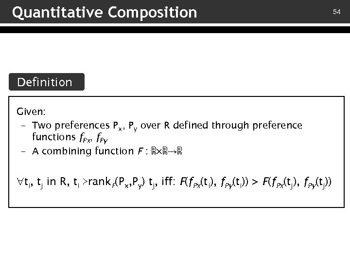
Quantitative Composition Definition Given: – Two preferences Px, Py over R defined through preference functions f. Px, f. Py – A combining function F : ℝ×ℝ→ℝ ti, tj in R, ti ≻rank. F(Px, Py) tj, iff: F(f. Px(ti), f. Py(ti)) > F(f. Px(tj), f. Py(tj)) 54

Quantitative Composition 55 To assign importance to preferences, weights can be used Example: P 1: f. P 1(ti)= 0. 001 × ti[duration] P 2: f. P 2(ti) = 0. 0001 × ti[year] rank. F(P 1, P 2): F(f. P 1(ti), f. P 2(ti)) = 0. 1 × f. P 1(ti) + 0. 9 × f. P 2(ti) Under this preference: score(t 1) = 0. 185 score(t 2) = 0. 187 score(t 3) = 0. 199 Also: Numerical composition over different relational schemas

Quantitative Composition 56 Other types of combining functions: – The min and max functions Three classes of combining functions: – Inflationary: the preference in a tuple increases with the number of preferences that satisfy it – Dominant: the most important preference dominates – Reserved: the preference in a tuple is between the highest and the lowest degrees of interest among the preferences satisfied [Koutrika and Ioannidis 2005 b]

Quantitative Composition 57 Preference Overriding Let Px, Py be two preferences defined over the relational schema R If Px refers to a subset of tuples that Py refers to, the more specific one, i. e. , Px, overrides the more generic one [Koutrika and Ioannidis 2010] Example: P 1: movie: (movie. genre = ‘comedy’, 0. 9) P 2: movie: (movie. genre = ‘comedy’ and movie. director = ‘Stiller’, 0. 9) P 2 overrides P 1 whenever they both apply

Qualitative vs. Quantitative Composition Note: Every composition mechanism defined over preference relations can be applied to preferences defined using functions or degrees of interest This way: – Prioritized, lexicographical, pareto, intersection, union and difference composition are also applicable to numerical preferences 58
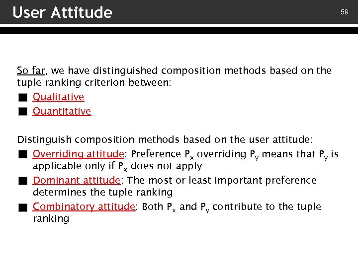
User Attitude So far, we have distinguished composition methods based on the tuple ranking criterion between: – Qualitative – Quantitative Distinguish composition methods based on the user attitude: – Overriding attitude: Preference Px overriding Py means that Py is applicable only if Px does not apply – Dominant attitude: The most or least important preference determines the tuple ranking – Combinatory attitude: Both Px and Py contribute to the tuple ranking 59
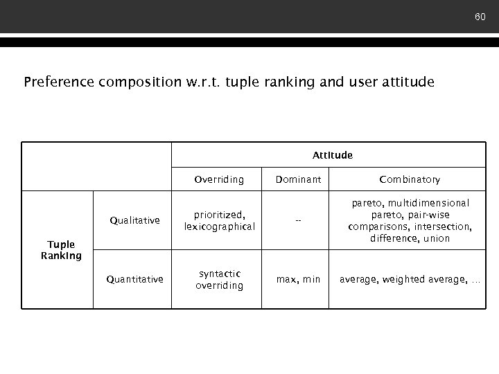
60 Preference composition w. r. t. tuple ranking and user attitude Attitude Overriding Dominant Combinatory Qualitative prioritized, lexicographical -- pareto, multidimensional pareto, pair-wise comparisons, intersection, difference, union Quantitative syntactic overriding max, min average, weighted average, … Tuple Ranking
Heterogeneous Composition So far, we have focused on: – Mechanisms for composing preferences for tuples Is this the only direction? Next, we focus on: – Combining preferences of different granularity 61

Heterogeneous Composition Mechanisms for composing preferences of different granularity Combine preferences expressed at tuple and relationship level Combine preferences expressed at tuple and attribute level 62
Heterogeneous Composition 63 Combine preferences expressed at tuple and relationship level To do this: Compose implicit preferences by other composeable ones Px and Py are composeable, iff: i. Px is a join preference of the form Rx: (qx, dx) connecting Rx to a relation Ry and ii. Py is a join or selection preference on Ry, i. e. , Ry: (qy, dy) [Koutrika and Ioannidis 2005 b] qx and qy are conditions, dx and dy are scores, Px and Py can be viewed as queries that select tuples from relations Rx, Ry that satisfy qx, qy

Heterogeneous Composition Combine preferences expressed at tuple and relationship level Example: Selection preference: actor: (actor. name = ‘Roberts’, 0. 8) Join preferences: movie: (movie. mid = play. mid, 1) play: (play. aid = actor. aid, 1) Implicit preference for movies with Julia Roberts: movie: (movie. mid = play. mid and play. aid = actor. aid and actor. name = ‘Roberts’, 0. 8) 64
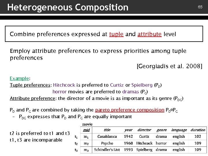
Heterogeneous Composition 65 Combine preferences expressed at tuple and attribute level Employ attribute preferences to express priorities among tuple preferences [Georgiadis et al. 2008] Example: Tuple preferences: Hitchcock is preferred to Curtiz or Spielberg (PD) horror movies are preferred to dramas (PG) Attribute preference: the director of a movie is as important as its genre (PDG) PD and PG are combined by taking the pareto preference composition PD⊗PG – PDG expresses that PD and PG are equally important t 2 is preferred to t 1 and t 3 t 1, t 3 are incomparable

Preference Composition: Summary 66 Preference composition w. r. t. granularity Tuple Relation Attribute Relationship [Agrawal and Wimmers 2000; Agrawal et al. 2006; Bunningen et al. 2006; 2007; Chomicki 2002; 2003; Georgiadis et al. 2008; Holland Kiessling 2004; Kiessling 2002; Koutrika and Ioannidis 2004; 2005 b; Miele et al. 2009; Stefanidis et al. 2006; 2007; Zhang and Chomicki 2008] Relation Attribute Relationship -- [Georgiadis et al. 2008] [Koutrika and Ioannidis 2004; 2005 b] -- -- -- [Georgiadis et al. 2008; Miele et al. 2009] -- [Koutrika and Ioannidis 2004; 2005 b]

Preferential Query Processing 67 Given a set of preferences: How we can employ them to compute query results? Goal: Exploit preferences to provide users with customized answers by changing the order and possibly the size of results

Tutorial Overview Preference Representation Preference Composition Preferential Query Processing Expand Database Queries with Preferences Preference Learning Pre-compute Rankings of Tuples Top-k Processing 68

Expand Database Queries 69 Three fundamental steps: v – Preference relatedness: determine which preferences are related and applicable to a query – v Preference filtering: identify which of the related preferences should be integrated into the query v – Preference integration: integrate the selected preferences into the original query to enable preferential query answering
Expand Database Queries Preference Relatedness From a set of preferences known for a user at query time: v – All preferences may be considered related to the query v – Only a subset of preferences may be considered related to the query Which of the available preferences we will use? 70
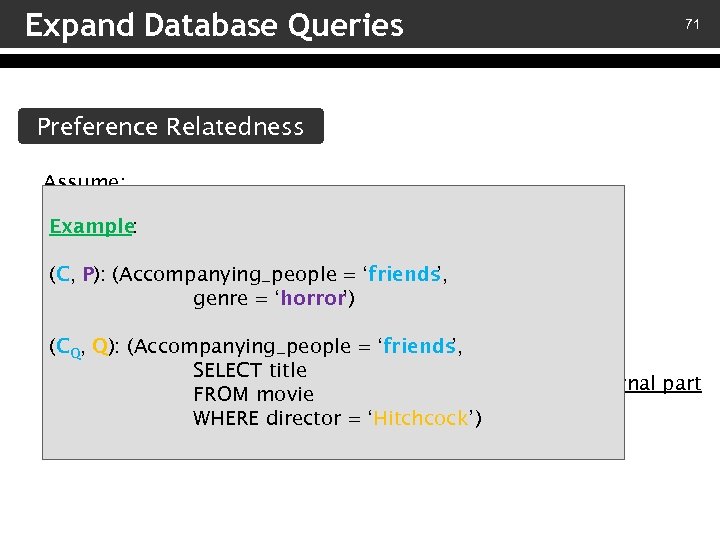
Expand Database Queries 71 Preference Relatedness Assume: – A preference (C, P) Example : o P is defined for C (C, o C (Accompanying_people = or null ’, P): can be internal, external ‘friends genre = ‘horror ’) – A query (CQ, Q) (CQo Q): is formulated over the database (internal part) , Q (Accompanying_people = ‘friends ’, SELECT title o CQ is described by the context parameters of the external part FROM movie of C WHERE director = ‘Hitchcock’) – CQ may be null if no external context is specified

Expand Database Queries 72 Preference Relatedness A preference (C, P) is related to a query (CQ, Q) if: – The external part of C matches CQ and the internal part of C matches Q – The preference part P is applicable to Q’s results In what follows, we elaborate each part of the definition separately: – Context matching – Preference applicability

Expand Queries: Preference Relatedness 73 Context Matching Use a metric for measuring the distance, similarity or difference of two contexts: v – Vector-based approaches o Represent query and preference contexts as vectors and measure their similarity [Agrawal et al. 2006] v – Hierarchical-based approaches
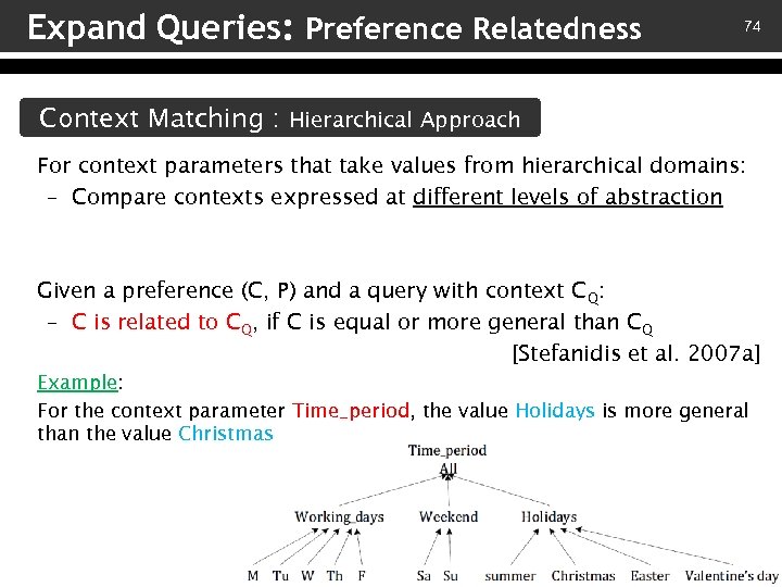
Expand Queries: Preference Relatedness 74 Context Matching : Hierarchical Approach For context parameters that take values from hierarchical domains: – Compare contexts expressed at different levels of abstraction Given a preference (C, P) and a query with context CQ: – C is related to CQ, if C is equal or more general than CQ [Stefanidis et al. 2007 a] Example: For the context parameter Time_period, the value Holidays is more general than the value Christmas

Expand Queries: Preference Relatedness 75 Context Matching : Hierarchical Approach Hierarchical distance Distance between C and CQ: Sum of distances of the levels of all context parameters – Distance between two levels: Minimum path between them in the hierarchy Example: The contexts (Athens, warm) and (Greece, good) have distance 1+1=2 Location ALL Weather ALL Continent Weather characterization (bad, good) Country City Conditions (freezing, cold, mild, warm, hot) A similar metric is used by [Miele et al. 2009] • Take into account the depth of context values in the hierarchy

Expand Queries: Preference Relatedness 76 Context Matching : Hierarchical Approach Locate the related preferences using the profile tree – Exploit the repetition of context values in contexts [Stefanidis et al. 2007 a] Preferences (C, P): • ((all, all), P 0) • ((friends, good, summer holidays), P 1) • ((family, good, summer holidays), P 2) • ((friends, all, holidays), P 3) • ((family, all, holidays), P 4) • ((family, all), P 5) • ((all, holidays), P 6) summer holidays P 1 friends good holidays p 3 all good all family all summer holidays p 2 all holidays p 4 all p 5 holidays p 6 all p 0
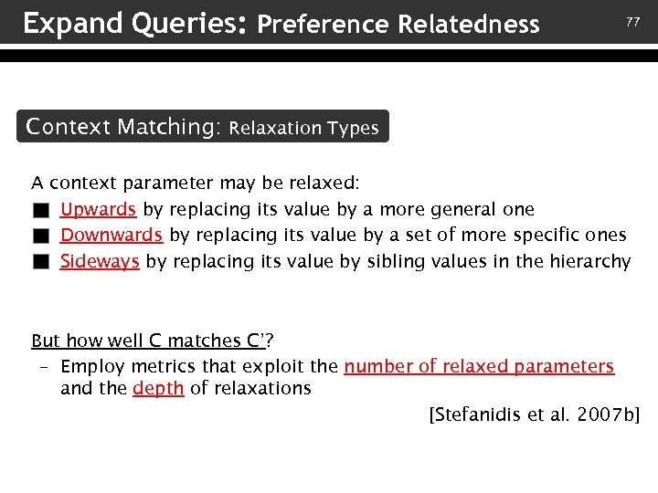
Expand Queries: Preference Relatedness 77 Context Matching: Relaxation Types A context parameter may be relaxed: – v Upwards by replacing its value by a more general one – v Downwards by replacing its value by a set of more specific ones v Sideways by replacing its value by sibling values in the hierarchy – But how well C matches C’? – Employ metrics that exploit the number of relaxed parameters and the depth of relaxations [Stefanidis et al. 2007 b]
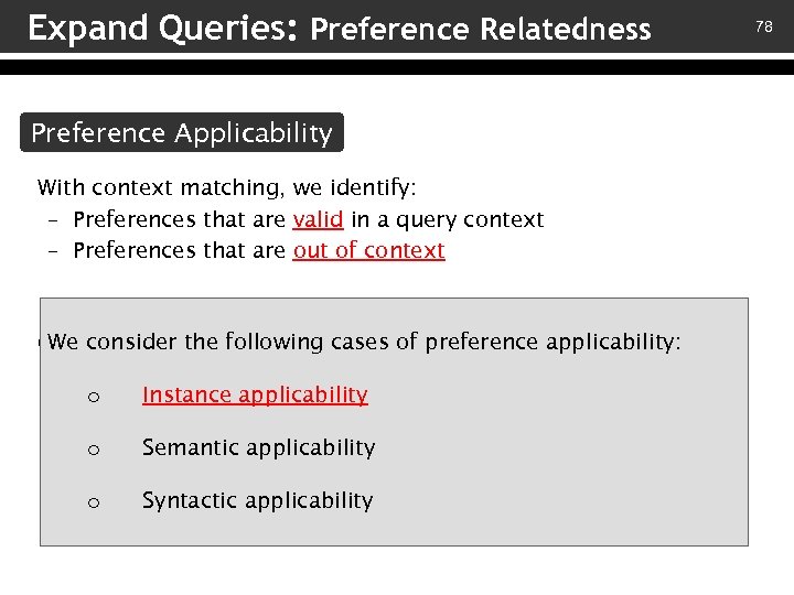
Expand Queries: Preference Relatedness Preference Applicability With context matching, we identify: – Preferences that are valid in a query context – Preferences that are out of context It does not guarantee that a preference can be combined with the query and yield an interesting, non-empty output We consider the following cases of preference applicability: o Instance applicability Little work has been done in this direction… o Semantic applicability o Syntactic applicability 78

Expand Queries: Preference Relatedness 79 Instance Applicability P is instantly applicable to Q if: Q, combined conjunctively with P, is executed over the current database instance and its result set is not empty Example: For a Q about recent movies and a P for movies directed by Spielberg: – P is instantly applicable to Q only if the database contains recent entries of Steven Spielberg

Expand Queries: Preference Relatedness Semantic Applicability For semantic applicability, additional knowledge, outside the database, is needed Example: For a Q about comedies: – A preference for movies directed by Allen is applicable – A preference for Tarkovsky is not applicable 80
Expand Queries: Preference Relatedness 81 Semantic Applicability For semantic applicability, additional knowledge, outside the database, is needed Note: When P is instantly applicable to Q, then P is also semantically applicable to Q – The reverse does not apply Example: For a Q about recent movies and a P for movies directed by Tarantino – P is semantically applicable to Q – Assuming that our database is not updated, P is not instantly applicable to Q

Expand Queries: Preference Relatedness 82 Syntactic Applicability A preference P is syntactically applicable to a query Q w. r. t. their structure – That is, according to the relations, attributes and values P and Q contain A P for the tuples of a relation R is applicable to Q, if: – R is referenced in Q – P is expressed over an attribute in Q [Koutrika and Ioannidis 2004] Examples: Note: – If Q returns movies starring Roberts, a P for Stiller is syntactically applicable, since a movie has many actors The set of semantically applicable preferences for a query is a – For a Q about movies after 2000, a P for movies superset of the syntactically applicable ones before 1990 is conflicting
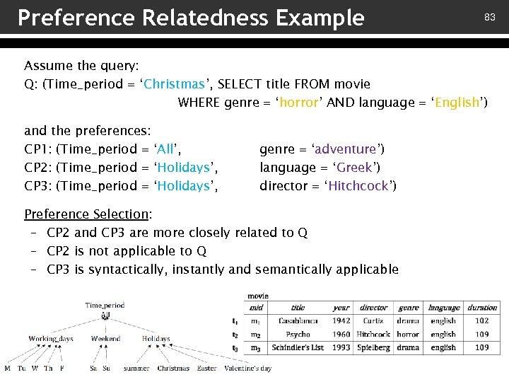
Preference Relatedness Example 83 Assume the query: Q: (Time_period = ‘Christmas’, SELECT title FROM movie WHERE genre = ‘horror’ AND language = ‘English’) and the preferences: CP 1: (Time_period = ‘All’, CP 2: (Time_period = ‘Holidays’, CP 3: (Time_period = ‘Holidays’, genre = ‘adventure’) language = ‘Greek’) director = ‘Hitchcock’) Preference Selection: – CP 2 and CP 3 are more closely related to Q – CP 2 is not applicable to Q – CP 3 is syntactically, instantly and semantically applicable
Expand Database Queries 84 Three fundamental steps: v – Preference relatedness: determine which preferences are related and applicable to a query – v Preference filtering: identify which of the related preferences should be integrated into the query v – Preference integration: integrate the selected preferences into the original query to enable preferential query answering
Expand Queries: Preference Filtering 85 All preferences related to a query may be used for ranking and selecting the tuples returned by the query Alternatively: Rank preferences based on their: – Relatedness score, capturing the degree to which a preference is related to a query – Preference score, showing their intensity Subsequently, select the top preferences for ranking the query results
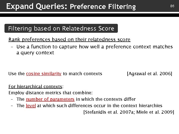
Expand Queries: Preference Filtering 86 Filtering based on Relatedness Score Rank preferences based on their relatedness score – Use a function to capture how well a preference context matches a query context Use the cosine similarity to match contexts [Agrawal et al. 2006] For hierarchical contexts: Employ distance metrics that combine: – The number of parameters in which the contexts differ – The level at which such differences occur in the context hierarchies [Stefanidis et al. 2007 a; Miele et al. 2009]
Expand Queries: Preference Filtering 87 Filtering based on Preference Score Quantitative preferences are ordered in decreasing preference score and the top K ones are selected for expanding the query

Expand Queries: Preference Filtering 88 Filtering based on Preference Score Extract the top K related preferences from a set U – These preferences are stored explicitly in U or are derived implicitly through preference composition [Koutrika and Ioannidis 2004] Example: Selection preference: actor: (actor. name = ‘Roberts’, 0. 8) Join preferences: movie: (movie. mid = play. mid, 1) play: (play. aid = actor. aid, 1) Implicit preference for movies with Julia Roberts: movie: (movie. mid = play. mid and play. aid = actor. aid and actor. name = ‘Roberts’, 0. 8)
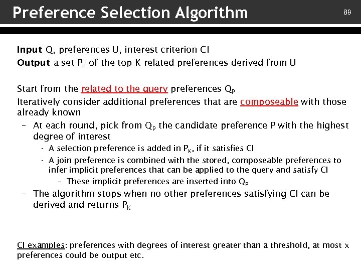
Preference Selection Algorithm 89 Input: Q, preferences U, interest criterion CI Output a set PK of the top K related preferences derived from U : Start from the related to the query preferences QP Iteratively consider additional preferences that are composeable with those already known – At each round, pick from QP the candidate preference P with the highest degree of interest • A selection preference is added in PK, if it satisfies CI • A join preference is combined with the stored, composeable preferences to infer implicit preferences that can be applied to the query and satisfy CI – These implicit preferences are inserted into QP – The algorithm stops when no other preferences satisfying CI can be derived and returns PK CI examples: preferences with degrees of interest greater than a threshold, at most x preferences could be output etc.

Expand Database Queries 90 Three fundamental steps: v – Preference relatedness: determine which preferences are related and applicable to a query – v Preference filtering: identify which of the related preferences should be integrated into the query v – Preference integration: integrate the selected preferences into the original query to enable preferential query answering

Expand Queries: Preference Integration 91 Preferences expressed as query conditions can be naturally integrated into a query – Query rewriting approaches leverage the power of SQL to return results that satisfy the user preferences Use the top K preferences for query personalization – Query results satisfy at least L of the K preferences o K: Desired degree of personalization o L: Minimum number of criteria that an answer should meet [Koutrika and Ioannidis 2004] Two different query re-writing mechanisms: i. Single query: A conjunction of query conditions with the disjunction of all possible conjunctions of the L out of K preferences ii. K queries: Augment the initial query with one of the K preferences o Each tuple that appears at least L times is output
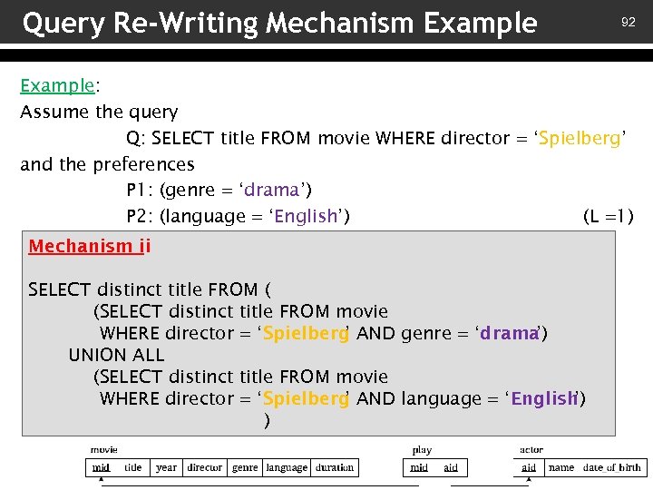
Query Re-Writing Mechanism Example 92 Example: Assume the query Q: SELECT title FROM movie WHERE director = ‘Spielberg’ and the preferences P 1: (genre = ‘drama’) P 2: (language = ‘English’) (L =1) Mechanism ii Mechanism i SELECT distinct title FROM ( (SELECT distinct title FROM movie SELECT title FROM movie WHERE director = ‘Spielberg AND ’ WHERE director = ‘Spielberg AND genre = ‘drama’) ’ (genre = ‘drama’ OR language = ‘English ’) UNION ALL (SELECT distinct title FROM movie WHERE director = ‘Spielberg AND language = ‘English ’ ’) )
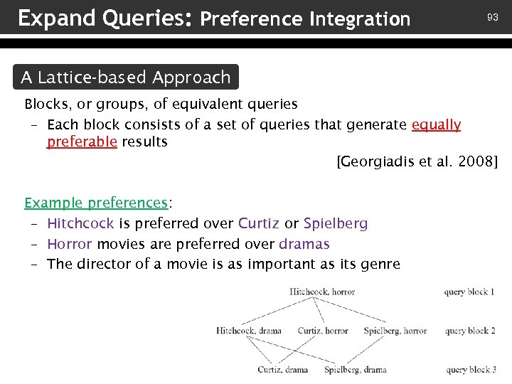
Expand Queries: Preference Integration 93 A Lattice-based Approach Blocks, or groups, of equivalent queries – Each block consists of a set of queries that generate equally preferable results [Georgiadis et al. 2008] Example preferences: – Hitchcock is preferred over Curtiz or Spielberg – Horror movies are preferred over dramas – The director of a movie is as important as its genre
Expand Database Queries: Summary 94 Three fundamental steps: v – Preference relatedness: determine which preferences are related and applicable to a query o All preferences o Context matching o Preference applicability v – Preference filtering: identify which of the related preferences should be integrated into the query o Preference relatedness o Preference score v – Preference integration: integrate the selected preferences into the original query to enable preferential query answering
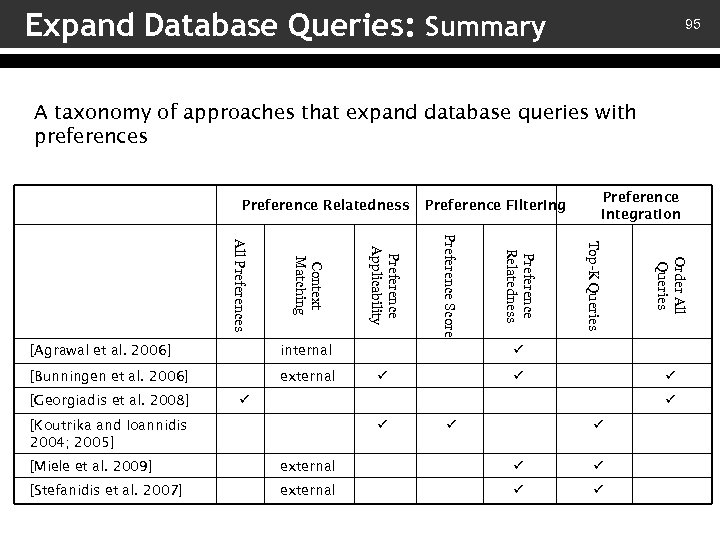
Expand Database Queries: Summary 95 A taxonomy of approaches that expand database queries with preferences Preference Relatedness Preference Integration Order All Queries Top-K Queries [Georgiadis et al. 2008] Preference Relatedness external Preference Score internal [Bunningen et al. 2006] Preference Applicability Context Matching All Preferences [Agrawal et al. 2006] Preference Filtering [Koutrika and Ioannidis 2004; 2005] [Miele et al. 2009] external [Stefanidis et al. 2007] external

Expand Database Queries Preference integration – Employ preference operators 96
Employ Preference Operators 97 Preferences can be embedded into query languages through preference-related operators – Select from input the set of the most preferred tuples Two fundamentals approaches to handle preference operators: v – Operator implementation o Operators are implemented inside the database engine – Employ special evaluation algorithmic techniques v – Operator translation o Operators are translated into other, existing relational algebra operators
Employ Preference Operators In following, we focus on: v – Defining preference operators v – Implementing preference operators v Translating preference operators – 98
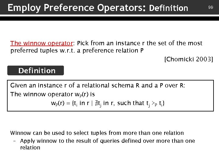
Employ Preference Operators: Definition 99 The winnow operator: Pick from an instance r the set of the most preferred tuples w. r. t. a preference relation P [Chomicki 2003] Definition Given an instance r of a relational schema R and a P over R: The winnow operator w. P(r) is w. P(r) = {ti in r | ∄tj in r, such that tj ≻P ti} Winnow can be used to select tuples from more than one relation – Apply winnow to the result of queries defined over more than one relation
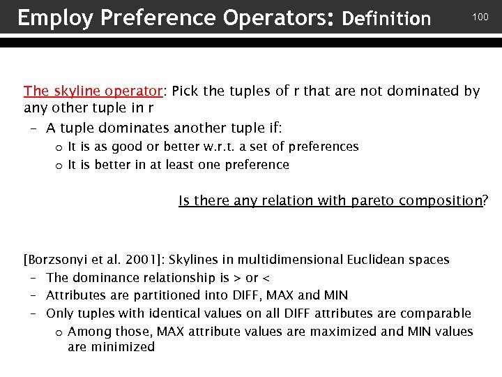
Employ Preference Operators: Definition 100 The skyline operator: Pick the tuples of r that are not dominated by any other tuple in r – A tuple dominates another tuple if: o It is as good or better w. r. t. a set of preferences o It is better in at least one preference Is there any relation with pareto composition? [Borzsonyi et al. 2001]: Skylines in multidimensional Euclidean spaces – The dominance relationship is > or < – Attributes are partitioned into DIFF, MAX and MIN – Only tuples with identical values on all DIFF attributes are comparable o Among those, MAX attribute values are maximized and MIN values are minimized
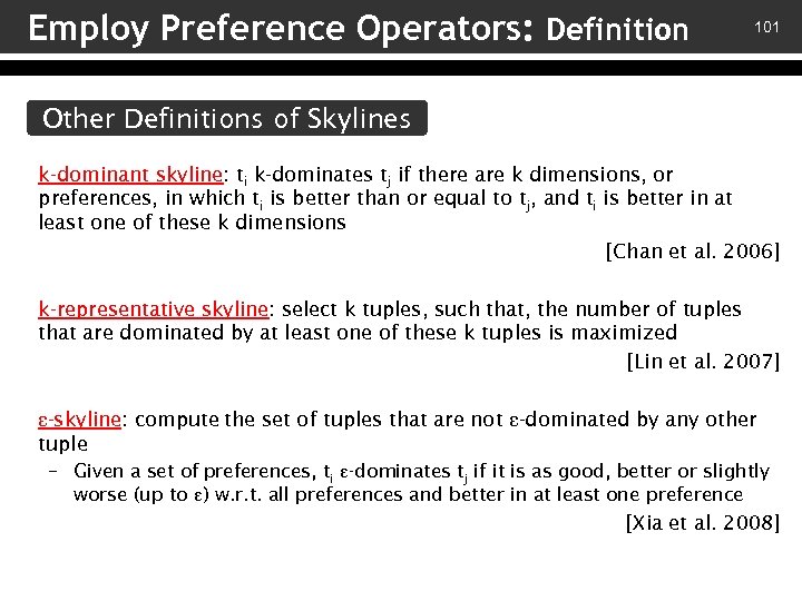
Employ Preference Operators: Definition 101 Other Definitions of Skylines k-dominant skyline: ti k-dominates tj if there are k dimensions, or preferences, in which ti is better than or equal to tj, and ti is better in at least one of these k dimensions [Chan et al. 2006] k-representative skyline: select k tuples, such that, the number of tuples that are dominated by at least one of these k tuples is maximized [Lin et al. 2007] ε-skyline: compute the set of tuples that are not ε-dominated by any other tuple – Given a set of preferences, ti ε-dominates tj if it is as good, better or slightly worse (up to ε) w. r. t. all preferences and better in at least one preference [Xia et al. 2008]
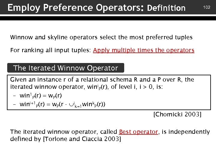
Employ Preference Operators: Definition 102 Winnow and skyline operators select the most preferred tuples For ranking all input tuples: Apply multiple times the operators The Iterated Winnow Operator Given an instance r of a relational schema R and a P over R, the iterated winnow operator, wini. P(r), of level i, i > 0, is: – win 1 P(r) = w. P(r) – wini+1 P(r) = w. P(r - ik=1 wink. P(r)) [Chomicki 2003] The iterated winnow operator, called Best operator, is independently defined by [Torlone and Ciaccia 2003]
Employ Preference Operators In following, we focus on: v – Defining preference operators v – Implementing preference operators v Translating preference operators – 103
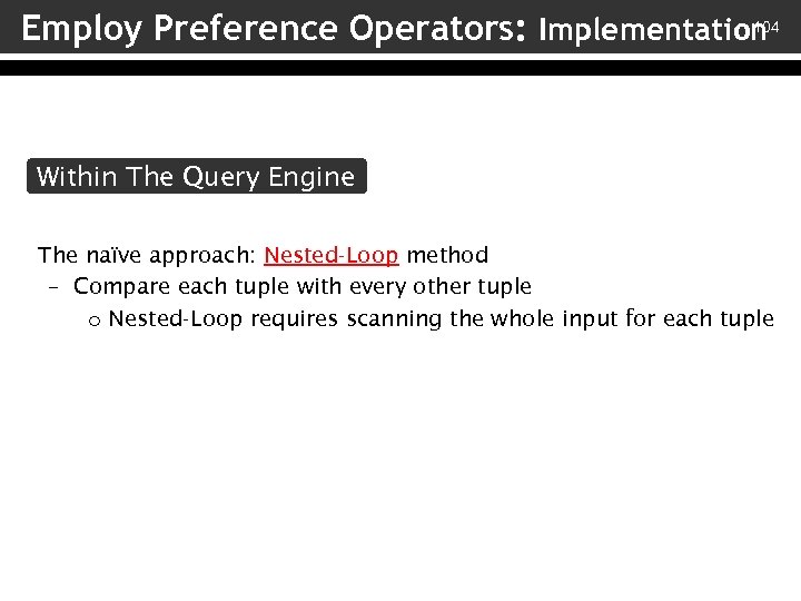
104 Employ Preference Operators: Implementation Within The Query Engine The naïve approach: Nested-Loop method – Compare each tuple with every other tuple o Nested-Loop requires scanning the whole input for each tuple
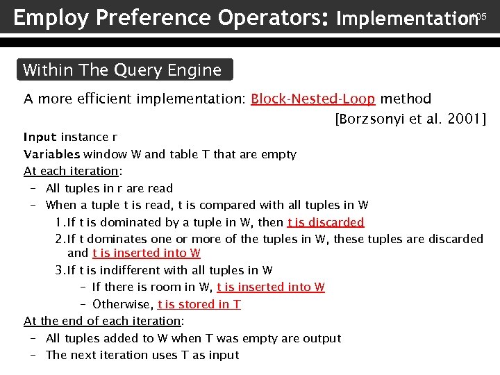
105 Employ Preference Operators: Implementation Within The Query Engine A more efficient implementation: Block-Nested-Loop method [Borzsonyi et al. 2001] Input: instance r Variables window W and table T that are empty : At each iteration: – All tuples in r are read – When a tuple t is read, t is compared with all tuples in W 1. If t is dominated by a tuple in W, then t is discarded 2. If t dominates one or more of the tuples in W, these tuples are discarded and t is inserted into W 3. If t is indifferent with all tuples in W – If there is room in W, t is inserted into W – Otherwise, t is stored in T At the end of each iteration: – All tuples added to W when T was empty are output – The next iteration uses T as input

106 Employ Preference Operators: Implementation Iterated winnow operator implementation – Apply one of the previous algorithms (e. g. , the NL or SFS) multiple times o First, apply on r to produce win 1 P(r) o Then, apply on (r - ik=1 wink. P(r)) to produce wini+1 P(r) Evaluating Best Operator algorithm [Torlone and Ciaccia 2003] BNL variation – Compute wini+1 P(r) from those tuples that were found to be directly dominated by a tuple in wini. P(r)
Employ Preference Operators In following, we focus on: v – Defining preference operators v – Implementing preference operators v Translating preference operators – 107
Employ Preference Operators: Translation 108 Is the only solution to implement preference operators? – Translate operators into existing relational algebra operators [Kießling 2002] defines preference queries with two new relational operators: 1. Preference selection operator: corresponds to the winnow operator w. P(r) 2. Grouped preference selection operator: apply preference selection within groups Given an attribute set B: o Tuples are partitioned into groups with same values in B o The grouped preference selection operator selects the dominating tuples in each group
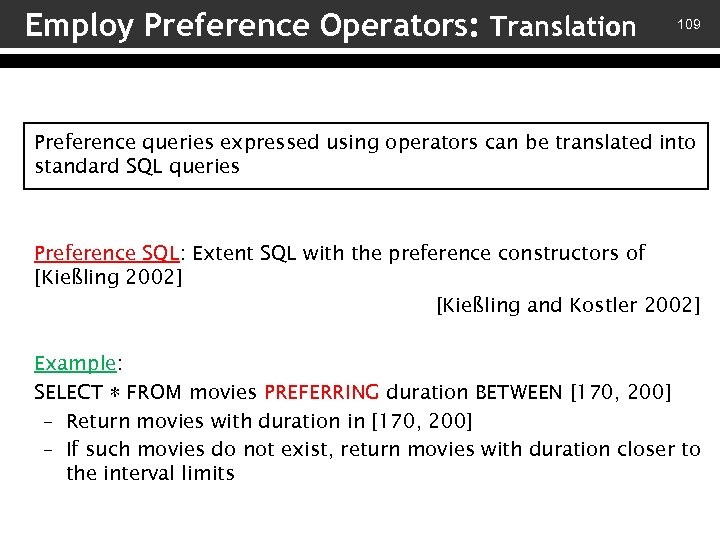
Employ Preference Operators: Translation 109 Preference queries expressed using operators can be translated into standard SQL queries Preference SQL: Extent SQL with the preference constructors of [Kießling 2002] [Kießling and Kostler 2002] Example: SELECT ∗ FROM movies PREFERRING duration BETWEEN [170, 200] – Return movies with duration in [170, 200] – If such movies do not exist, return movies with duration closer to the interval limits
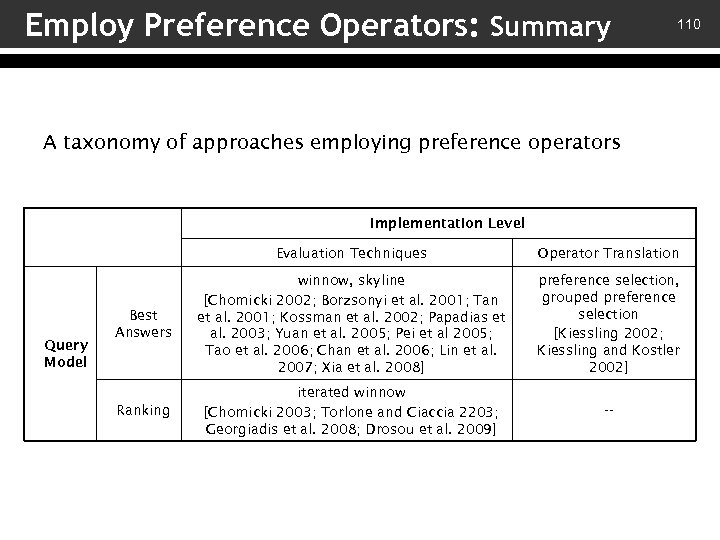
Employ Preference Operators: Summary 110 A taxonomy of approaches employing preference operators Implementation Level Evaluation Techniques Query Model Operator Translation Best Answers winnow, skyline [Chomicki 2002; Borzsonyi et al. 2001; Tan et al. 2001; Kossman et al. 2002; Papadias et al. 2003; Yuan et al. 2005; Pei et al 2005; Tao et al. 2006; Chan et al. 2006; Lin et al. 2007; Xia et al. 2008] preference selection, grouped preference selection [Kiessling 2002; Kiessling and Kostler 2002] Ranking iterated winnow [Chomicki 2003; Torlone and Ciaccia 2203; Georgiadis et al. 2008; Drosou et al. 2009] --
Expand Database Queries: Summary 111 Numerous evaluation methods for preference queries – Only a few are implemented within the core of a database system Flex. Pref: A framework for extensible preference evaluation in database systems Integration with Flex. Pref: register the functions that implement a preference method – Once integrated, the preference method “lives” at the core of the database [Levandoski et al. 2010]
Preferential Query Processing 112 Preferential query processing methods: v – Expand regular database queries with preferences v – Pre-compute rankings of database tuples based on preferences v Top-k processing –
Pre-compute Rankings 113 Perform some pre-processing offline to make online processing of queries fast How? – Employ preferences to construct offline representative rankings – At query time, select the relevant rankings and use them to report results We organize existing approaches into: v Context-based approaches – v Context-free approaches –

114 Pre-compute Rankings: Context-based Approaches Pre-compute representative rankings of database tuples based on contextual preferences But how the representative rankings are constructed?
![115 Pre-compute Rankings: Context-based Approaches [Agrawal et al. 2006] – Construct a ranking for 115 Pre-compute Rankings: Context-based Approaches [Agrawal et al. 2006] – Construct a ranking for](https://present5.com/presentation/10293420997c01f00f6142a677539b01/image-115.jpg)
115 Pre-compute Rankings: Context-based Approaches [Agrawal et al. 2006] – Construct a ranking for each set of preferences with the same context – Maintain only a set of representative rankings How to select the representative rankings? v Greedy Algorithm – o Begin from all rankings o Remove at each step the ranking that is the most similar to the remaining ones v Furthest Algorithm – o Select randomly a ranking o At each step, pick the ranking which is furthest from the already selected ones o Continue up to collect the desirable number of representative rankings The distance between two rankings may be computed using either the Spearman footrule or the Kendall tau distance
![116 Pre-compute Rankings: Context-based Approaches [Stefanidis and Pitoura 2008] – Create groups of similar 116 Pre-compute Rankings: Context-based Approaches [Stefanidis and Pitoura 2008] – Create groups of similar](https://present5.com/presentation/10293420997c01f00f6142a677539b01/image-116.jpg)
116 Pre-compute Rankings: Context-based Approaches [Stefanidis and Pitoura 2008] – Create groups of similar preferences – Construct a ranking for each group Which preferences are similar? v Contextual clustering – o Consider as similar the preferences with similar context v – Predicate clustering o Consider as similar the preferences with similar predicates and scores
117 Pre-compute Rankings: Context-free Approaches Such approaches employ materialized preference views – Relational views ordered according to a preference, or scoring, function Main goal: Locate the k results that maximize (or minimize) a combining preference function in a pipelined manner e. g. , [Hristidis and Papakonstantinou 2004]

Pre-computing Rankings: Summary 118 A taxonomy of pre-computing rankings approaches Context-based Context-free Qualitative [Agrawal et al. 2006] -- Quantitative [Stefanidis and Pitoura 2008; You and Hwang 2008] [Hristidis and Papakonstantinou 2004; Das et al. 2006; Yi et al. 2003] Formulation
Preferential Query Processing 119 Preferential query processing methods: v – Expand regular database queries with preferences v – Pre-compute rankings of database tuples based on preferences v Top-k processing –
Top-k Processing Top-k query: provide the k most important results Basic Idea – Assign scores to all tuples based on a scoring function or an aggregation of a set of functions – Report the k tuples with the highest scores 120

Top-k Processing Previous Week! 121

Top-k Processing 122 Above: Aggregate rankings that contain the same set of tuples – The produced ranking consists of the same tuple set Top-k Joined Tuples Report the k joined tuples with the largest interest scores – Tuples of different rankings are joined w. r. t. specific join conditions – Each tuple has a score computed from the scores of the participating tuples [Natsev et al. 2001; Ilyas et al. 2004] Top-k Groups of Tuples Report the k groups of tuples with the largest interest scores – Scores are computed using a group aggregation function [Li et al. 2006]

Top-k Processing: Summary 123 A taxonomy of top-k query processing techniques Implementation Level Application level Top-k tuples Query Model Within engine [Fagin et al. 2001; Nepal and Ramakrishna 1999; Guntzer et al. 2000] -- Top-k joined tuples [Natsev et al. 2001] [Ilyas et al. 2004] Top-k groups of tuples -- [Li et al. 2006]
Tutorial Overview Preference Representation Preference Composition Preferential Query Processing Preference Learning 124
Conclusions Preference Representation Preference Composition Preferential Query Processing 125
Conclusions Preference Representation Existing methods are divided into qualitative and quantitative Preference Composition Existing methods tackle specific aspects of the problem A holistic preference representation approach is missing Preferential Query Processing Complete understanding of user preferences is missing – (psychology? ) New types of preferenes 126
Conclusions Preference Representation Preference Composition Existing works follow a uniform approach to representation and composition Qualitative composition applies to preferences represented in either way Most approaches deal with tuple-to-tuple preference composition There are combinations that have not been touched at all Can composition be used as a means to resolve conflicts? Preferential Query Processing 127

Conclusions 128 Preference Representation Preference Composition Preferential Query Processing An approach for matching both internal and external preference context to query context is missing Approaches that deal with instance and semantic applicability are missing Embed preferences in the database Query + Preferences = ?
Future Directions Hybrid preference models Combining qualitative and quantitative aspects Group preferences Merging individual preferences [Amer-Yahia et al. 2009] Social preferences User preferences over the social graph 129
Future Directions Leveraging the wisdom of crowds Learning preferences Preference-aware query engine Making preferences first-class citizens Holistic optimizer 130

The End 131

References 132 1. Agrawal, R. , Rantzau, R. , and Terzi, E. 2006. Context-sensitive ranking. In SIGMOD. 383 – 394. 2. Agrawal, R. and Wimmers, E. L. 2000. A framework for expressing and combining preferences. In SIGMOD. 297– 306. 3. Aho, A. , Sagiv, Y. , and Ullman, J. D. 1979. Equivalence of relational expressions. SIAM J. of Computing 8, 2, 218– 246. 4. Amer-Yahia, S. , Roy, S. B. , Chawla, A. , Das, G. , and Yu, C. 2009. Group recommendation: Semantics and efficiency. PVLDB 2, 1, 754– 765. 5. Bolchini, C. , Curino, C. , Quintarelli, E. , Schreiber, F. A. , and Tanca, L. 2007. A dataoriented survey of context models. SIGMOD Record 36, 4, 19– 26. 6. Borda, J. -C. 1781. Mémoire sur les élections au scrutin. Histoire de l’ Académie Royale des Sciences. 7. Borzsonyi, S. , Kossmann, D. , and Stocker, K. 2001. The skyline operator. In ICDE. 421– 430. 8. Boutilier, C. , Brafman, R. I. , Hoos, H. H. , and Poole, D. 1999. Reasoning with conditional ceteris paribus preference statements. In Sym. on Uncertainty in AI. 71– 80. 9. Brown, P. , Bovey, J. , and Chen, X. 1997. Context-aware applications: From the laboratory to the marketplace. IEEE Personal Communications 4, 5, 5864. 10. Bunningen, A. H. , Feng, L. , and Apers, P. M. G. 2006. A context-aware preference model for database querying in an ambient intelligent environment. In DEXA. 33– 43.

References 133 11. Chan, C. Y. , Jagadish, H. V. , Tan, K. -L. , Tung, A. K. H. , and Zhang, Z. 2006. Finding kdominant skylines in high dimensional space. In SIGMOD. 503– 514. 12. Chekuri, C. and Rajaraman, A. 1997. Conjunctive query containment revisited. In ICDT. 56– 70. 13. Chen, G. and Kotz, D. 2000. A Survey of Context-Aware Mobile Computing Research. Tech. Rep. TR 2000 -381, Dartmouth College, Computer Science. November. 14. Chomicki, J. 2002. Querying with intrinsic preferences. In EDBT. 34– 51. 15. Chomicki, J. 2003. Preference formulas in relational queries. ACM Trans. Database Syst. 28, 4, 427– 466. 16. Chomicki, J. 2007. Semantic optimization techniques for preference queries. Inf. Syst. 32, 5, 670– 684. 17. Chomicki, J. , Godfrey, P. , Gryz, J. , and Liang, D. 2003. Skyline with presorting. In ICDE. 717– 719. 18. Condorcet, J. A. N. 1785. Essai Sur L’ application De L’ analyse a La Probabilité Des Décisions Rendues a La Pluralité Des Voix. Kessinger Publishing. 19. Das, G. , Gunopulos, D. , Koudas, N. , and Tsirogiannis, D. 2006. Answering top-k queries using views. In VLDB. 451– 462. 20. Delgrande, J. P. , Schaub, T. , and Tompits, H. 2003. A framework for compiling preferences in logic programs. TPLP 3, 2, 129– 187. 21. Dey, A. K. 2001. Understanding and using context. Personal Ubiquitous Comput. 5, 1, 4– 7.
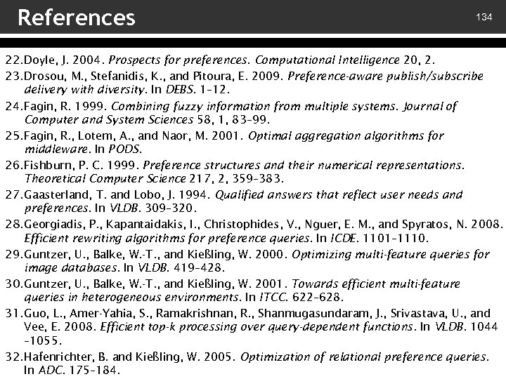
References 134 22. Doyle, J. 2004. Prospects for preferences. Computational Intelligence 20, 2. 23. Drosou, M. , Stefanidis, K. , and Pitoura, E. 2009. Preference-aware publish/subscribe delivery with diversity. In DEBS. 1– 12. 24. Fagin, R. 1999. Combining fuzzy information from multiple systems. Journal of Computer and System Sciences 58, 1, 83– 99. 25. Fagin, R. , Lotem, A. , and Naor, M. 2001. Optimal aggregation algorithms for middleware. In PODS. 26. Fishburn, P. C. 1999. Preference structures and their numerical representations. Theoretical Computer Science 217, 2, 359– 383. 27. Gaasterland, T. and Lobo, J. 1994. Qualified answers that reflect user needs and preferences. In VLDB. 309– 320. 28. Georgiadis, P. , Kapantaidakis, I. , Christophides, V. , Nguer, E. M. , and Spyratos, N. 2008. Efficient rewriting algorithms for preference queries. In ICDE. 1101– 1110. 29. Guntzer, U. , Balke, W. -T. , and Kießling, W. 2000. Optimizing multi-feature queries for image databases. In VLDB. 419– 428. 30. Guntzer, U. , Balke, W. -T. , and Kießling, W. 2001. Towards efficient multi-feature queries in heterogeneous environments. In ITCC. 622– 628. 31. Guo, L. , Amer-Yahia, S. , Ramakrishnan, R. , Shanmugasundaram, J. , Srivastava, U. , and Vee, E. 2008. Efficient top-k processing over query-dependent functions. In VLDB. 1044 – 1055. 32. Hafenrichter, B. and Kießling, W. 2005. Optimization of relational preference queries. In ADC. 175– 184.
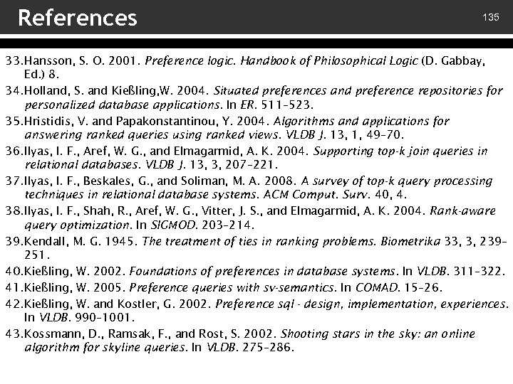
References 135 33. Hansson, S. O. 2001. Preference logic. Handbook of Philosophical Logic (D. Gabbay, Ed. ) 8. 34. Holland, S. and Kießling, W. 2004. Situated preferences and preference repositories for personalized database applications. In ER. 511– 523. 35. Hristidis, V. and Papakonstantinou, Y. 2004. Algorithms and applications for answering ranked queries using ranked views. VLDB J. 13, 1, 49– 70. 36. Ilyas, I. F. , Aref, W. G. , and Elmagarmid, A. K. 2004. Supporting top-k join queries in relational databases. VLDB J. 13, 3, 207– 221. 37. Ilyas, I. F. , Beskales, G. , and Soliman, M. A. 2008. A survey of top-k query processing techniques in relational database systems. ACM Comput. Surv. 40, 4. 38. Ilyas, I. F. , Shah, R. , Aref, W. G. , Vitter, J. S. , and Elmagarmid, A. K. 2004. Rank-aware query optimization. In SIGMOD. 203– 214. 39. Kendall, M. G. 1945. The treatment of ties in ranking problems. Biometrika 33, 3, 239– 251. 40. Kießling, W. 2002. Foundations of preferences in database systems. In VLDB. 311– 322. 41. Kießling, W. 2005. Preference queries with sv-semantics. In COMAD. 15– 26. 42. Kießling, W. and Kostler, G. 2002. Preference sql - design, implementation, experiences. In VLDB. 990– 1001. 43. Kossmann, D. , Ramsak, F. , and Rost, S. 2002. Shooting stars in the sky: an online algorithm for skyline queries. In VLDB. 275– 286.
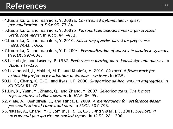
References 136 44. Koutrika, G. and Ioannidis, Y. 2005 a. Constrained optimalities in query personalization. In SIGMOD. 73– 84. 45. Koutrika, G. and Ioannidis, Y. 2005 b. Personalized queries under a generalized preference model. In ICDE. 841– 852. 46. Koutrika, G. and Ioannidis, Y. 2010. Answering queries based on preference hierarchies. TODS. 47. Koutrika, G. and Ioannidis, Y. E. 2004. Personalization of queries in database systems. In ICDE. 597– 608. 48. Lacroix, M. and Lavency, P. 1987. Preferences: putting more knowledge into queries. In VLDB. 217– 225. 49. Levandoski, J. , Mokbel, M. F. , and Khalefa, M. 2010. Flexpref: A framework for extensible preference evaluation in database systems. In ICDE. 50. Li, C. , Chang, K. C. -C. , and Ilyas, I. F. 2006. Supporting ad-hoc ranking aggregates. In SIGMOD. 61– 72. 51. Lin, X. , Yuan, Y. , Zhang, Q. , and Zhang, Y. 2007. Selecting stars: The k most representative skyline operator. In ICDE. 86– 95. 52. Miele, A. , Quintarelli, E. , and Tanca, L. 2009. A methodology for preference-based personalization of contextual data. In EDBT. 287– 298. 53. Natsev, A. , Chang, Y. -C. , Smith, J. R. , Li, C. -S. , and Vitter, J. S. 2001. Supporting incremental join queries on ranked inputs. In VLDB. 281– 290.
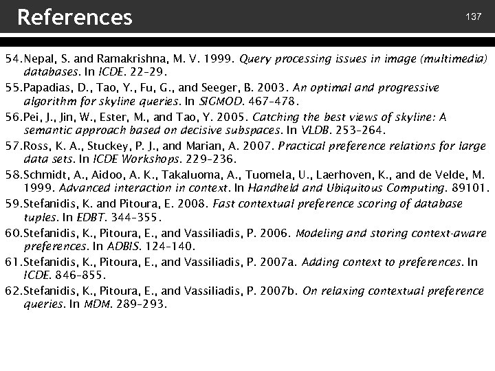
References 137 54. Nepal, S. and Ramakrishna, M. V. 1999. Query processing issues in image (multimedia) databases. In ICDE. 22– 29. 55. Papadias, D. , Tao, Y. , Fu, G. , and Seeger, B. 2003. An optimal and progressive algorithm for skyline queries. In SIGMOD. 467– 478. 56. Pei, J. , Jin, W. , Ester, M. , and Tao, Y. 2005. Catching the best views of skyline: A semantic approach based on decisive subspaces. In VLDB. 253– 264. 57. Ross, K. A. , Stuckey, P. J. , and Marian, A. 2007. Practical preference relations for large data sets. In ICDE Workshops. 229– 236. 58. Schmidt, A. , Aidoo, A. K. , Takaluoma, A. , Tuomela, U. , Laerhoven, K. , and de Velde, M. 1999. Advanced interaction in context. In Handheld and Ubiquitous Computing. 89101. 59. Stefanidis, K. and Pitoura, E. 2008. Fast contextual preference scoring of database tuples. In EDBT. 344– 355. 60. Stefanidis, K. , Pitoura, E. , and Vassiliadis, P. 2006. Modeling and storing context-aware preferences. In ADBIS. 124– 140. 61. Stefanidis, K. , Pitoura, E. , and Vassiliadis, P. 2007 a. Adding context to preferences. In ICDE. 846– 855. 62. Stefanidis, K. , Pitoura, E. , and Vassiliadis, P. 2007 b. On relaxing contextual preference queries. In MDM. 289– 293.
References 138 63. Tan, K. -L. , Eng, P. -K. , and Ooi, B. C. 2001. Efficient progressive skyline computation. In VLDB. 301– 310. 64. Tao, Y. , Xiao, X. , and Pei, J. 2006. Subsky: Efficient computation of skylines in subspaces. In ICDE. 65. Torlone, R. and Ciaccia, P. 2002. Finding the best when it’s a matter of preference. In SEBD. 347– 360. 66. Torlone, R. and Ciaccia, P. 2003. Management of user preferences in data intensive applications. In SEBD. 257– 268. 67. Vee, E. , Srivastava, U. , Shanmugasundaram, J. , Bhat, P. , and Amer-Yahia, S. 2008. Efficient computation of diverse query results. In ICDE. 228– 236. 68. Wellman, M. P. and Doyle, J. 1991. Preferential semantics for goals. AAAI. 698703. 69. Xia, T. , Zhang, D. , and Tao, Y. 2008. On skylining with flexible dominance relation. In ICDE. 1397– 1399. 70. Yi, K. , Yu, H. , Yang, J. , Xia, G. , and Chen, Y. 2003. Efficient maintenance of materialized top-k views. In ICDE. 189– 200. 71. You, G. and Hwang, S. 2008. Search structures and algorithms for personalized ranking. Information Sciences 178, 20, 3925– 3942. 72. Yuan, Y. , Lin, X. , Liu, Q. , Wang, W. , Yu, J. X. , and Zhang, Q. 2005. Efficient computation of the skyline cube. In VLDB. 241– 252. 73. Zhang, X. and Chomicki, J. 2008. Profiling sets for preference querying. In SEBD. 34– 44.
10293420997c01f00f6142a677539b01.ppt