Data Warehousing and Data Mining Chapter 7

Data Warehousing and Data Mining — Chapter 7 — MIS 542 2013 -2014 Fall 1

Chapter 7. Classification and Prediction n n What is classification? What is prediction? Issues regarding classification and prediction Classification by decision tree induction Bayesian Classification by Neural Networks Classification by Support Vector Machines (SVM) Classification based on concepts from association rule mining Other Classification Methods Prediction Classification accuracy Summary 2

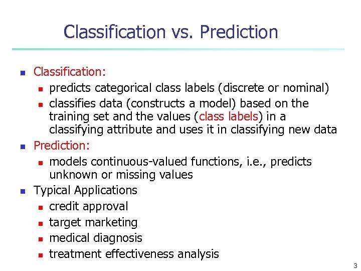Classification vs. Prediction n Classification: n predicts categorical class labels (discrete or nominal) n classifies data (constructs a model) based on the training set and the values (class labels) in a classifying attribute and uses it in classifying new data Prediction: n models continuous-valued functions, i. e. , predicts unknown or missing values Typical Applications n credit approval n target marketing n medical diagnosis n treatment effectiveness analysis 3

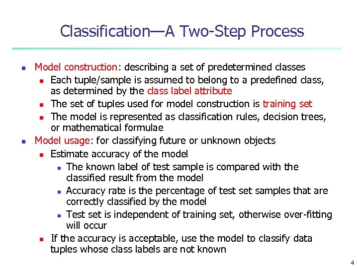Classification—A Two-Step Process n n Model construction: describing a set of predetermined classes n Each tuple/sample is assumed to belong to a predefined class, as determined by the class label attribute n The set of tuples used for model construction is training set n The model is represented as classification rules, decision trees, or mathematical formulae Model usage: for classifying future or unknown objects n Estimate accuracy of the model n The known label of test sample is compared with the classified result from the model n Accuracy rate is the percentage of test set samples that are correctly classified by the model n Test set is independent of training set, otherwise over-fitting will occur n If the accuracy is acceptable, use the model to classify data tuples whose class labels are not known 4

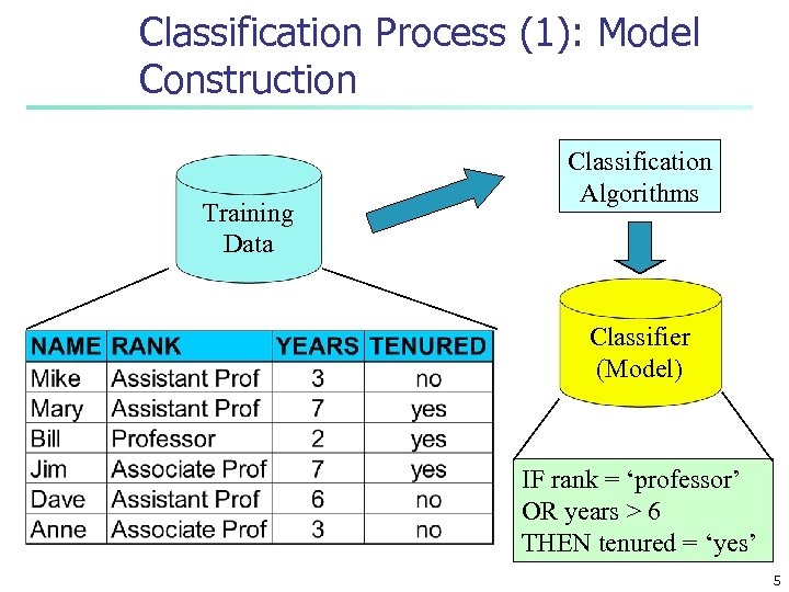Classification Process (1): Model Construction Training Data Classification Algorithms Classifier (Model) IF rank = ‘professor’ OR years > 6 THEN tenured = ‘yes’ 5

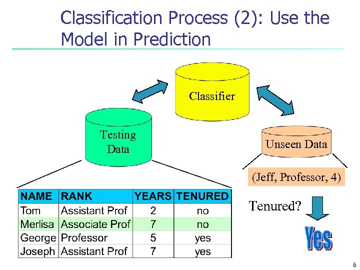Classification Process (2): Use the Model in Prediction Classifier Testing Data Unseen Data (Jeff, Professor, 4) Tenured? 6

Supervised vs. Unsupervised Learning n Supervised learning (classification) n n n Supervision: The training data (observations, measurements, etc. ) are accompanied by labels indicating the class of the observations New data is classified based on the training set Unsupervised learning (clustering) n n The class labels of training data is unknown Given a set of measurements, observations, etc. with the aim of establishing the existence of classes or clusters in the data 7

Chapter 7. Classification and Prediction n n What is classification? What is prediction? Issues regarding classification and prediction Classification by decision tree induction Bayesian Classification by Neural Networks Classification by Support Vector Machines (SVM) Classification based on concepts from association rule mining Other Classification Methods Prediction Classification accuracy Summary 8

Issues Regarding Classification and Prediction (1): Data Preparation n Data cleaning n n Relevance analysis (feature selection) n n Preprocess data in order to reduce noise and handle missing values Remove the irrelevant or redundant attributes Data transformation n Generalize and/or normalize data 9

Issues regarding classification and prediction (2): Evaluating Classification Methods n n n Predictive accuracy Speed and scalability n time to construct the model n time to use the model Robustness n handling noise and missing values Scalability n efficiency in disk-resident databases Interpretability: n understanding and insight provided by the model Goodness of rules n decision tree size n compactness of classification rules 10

Chapter 7. Classification and Prediction n n What is classification? What is prediction? Issues regarding classification and prediction Classification by decision tree induction Bayesian Classification by Neural Networks Classification by Support Vector Machines (SVM) Classification based on concepts from association rule mining Other Classification Methods Prediction Classification accuracy Summary 11

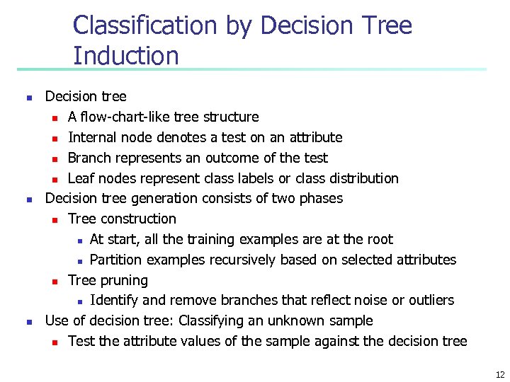Classification by Decision Tree Induction n Decision tree n A flow-chart-like tree structure n Internal node denotes a test on an attribute n Branch represents an outcome of the test n Leaf nodes represent class labels or class distribution Decision tree generation consists of two phases n Tree construction n At start, all the training examples are at the root n Partition examples recursively based on selected attributes n Tree pruning n Identify and remove branches that reflect noise or outliers Use of decision tree: Classifying an unknown sample n Test the attribute values of the sample against the decision tree 12

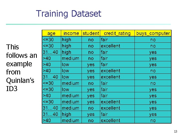Training Dataset This follows an example from Quinlan’s ID 3 13

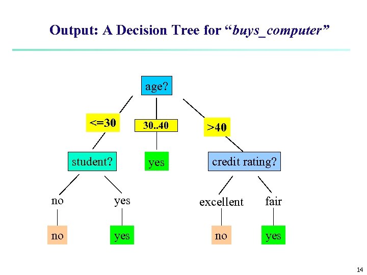Output: A Decision Tree for “buys_computer” age? <=30 student? overcast 30. . 40 yes >40 credit rating? no yes excellent fair no yes 14

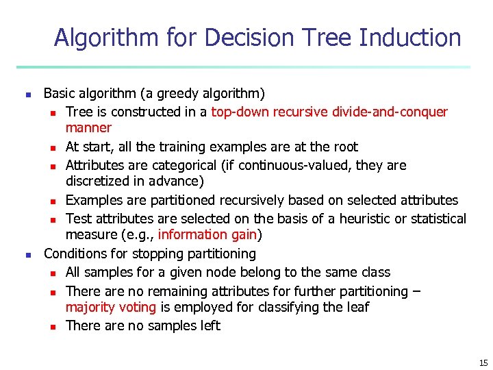Algorithm for Decision Tree Induction n n Basic algorithm (a greedy algorithm) n Tree is constructed in a top-down recursive divide-and-conquer manner n At start, all the training examples are at the root n Attributes are categorical (if continuous-valued, they are discretized in advance) n Examples are partitioned recursively based on selected attributes n Test attributes are selected on the basis of a heuristic or statistical measure (e. g. , information gain) Conditions for stopping partitioning n All samples for a given node belong to the same class n There are no remaining attributes for further partitioning – majority voting is employed for classifying the leaf n There are no samples left 15

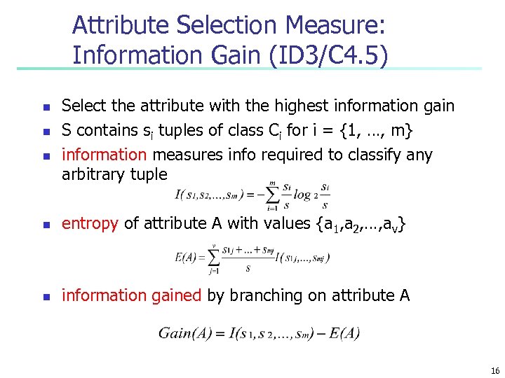Attribute Selection Measure: Information Gain (ID 3/C 4. 5) n n n Select the attribute with the highest information gain S contains si tuples of class Ci for i = {1, …, m} information measures info required to classify any arbitrary tuple n entropy of attribute A with values {a 1, a 2, …, av} n information gained by branching on attribute A 16

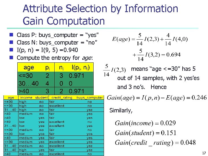Attribute Selection by Information Gain Computation Class P: buys_computer = “yes” g Class N: buys_computer = “no” g I(p, n) = I(9, 5) =0. 940 g Compute the entropy for age: g means “age <=30” has 5 out of 14 samples, with 2 yes’es and 3 no’s. Hence Similarly, 17

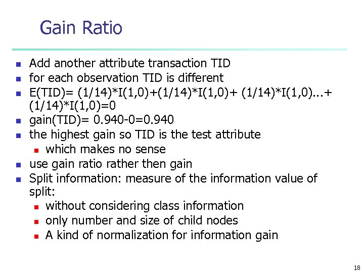Gain Ratio n n n n Add another attribute transaction TID for each observation TID is different E(TID)= (1/14)*I(1, 0)+ (1/14)*I(1, 0). . . + (1/14)*I(1, 0)=0 gain(TID)= 0. 940 -0=0. 940 the highest gain so TID is the test attribute n which makes no sense use gain ratio rather then gain Split information: measure of the information value of split: n without considering class information n only number and size of child nodes n A kind of normalization for information gain 18

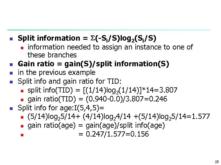n n n Split information = (-Si/S)log 2(Si/S) n information needed to assign an instance to one of these branches Gain ratio = gain(S)/split information(S) in the previous example Split info and gain ratio for TID: n split info(TID) = [(1/14)log 2(1/14)]*14=3. 807 n gain ratio(TID) = (0. 940 -0. 0)/3. 807=0. 246 Split info for age: I(5, 4, 5)= n (5/14)log 25/14+ (4/14)log 24/14 +(5/14)log 25/14=1. 577 n gain ratio(age) = gain(age)/split info(age) n = 0. 247/1. 577=0. 156 19

Exercise n Repeat the same exercise of constructing the tree by the gain ratio criteria as the attribute selection measure n notice that TID has the highest gain ratio n do not split by TID 20

Other Attribute Selection Measures n Gini index (CART, IBM Intelligent. Miner) n n All attributes are assumed continuous-valued Assume there exist several possible split values for each attribute May need other tools, such as clustering, to get the possible split values Can be modified for categorical attributes 21

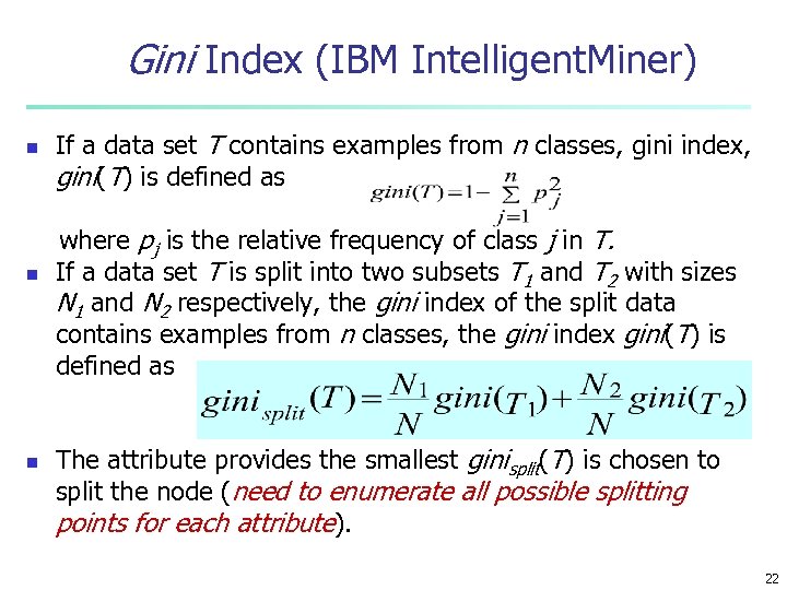Gini Index (IBM Intelligent. Miner) n n n If a data set T contains examples from n classes, gini index, gini(T) is defined as where pj is the relative frequency of class j in T. If a data set T is split into two subsets T 1 and T 2 with sizes N 1 and N 2 respectively, the gini index of the split data contains examples from n classes, the gini index gini(T) is defined as The attribute provides the smallest ginisplit(T) is chosen to split the node (need to enumerate all possible splitting points for each attribute). 22

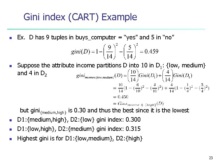Gini index (CART) Example n n Ex. D has 9 tuples in buys_computer = “yes” and 5 in “no” Suppose the attribute income partitions D into 10 in D 1: {low, medium} and 4 in D 2 but gini{medium, high} is 0. 30 and thus the best since it is the lowest n D 1: {medium, high}, D 2: {low} gini index: 0. 300 n D 1: {low, high}, D 2: {medium} gini index: 0. 315 n Highest gini is for D 1: {low, medium}, D 2: {high} 23

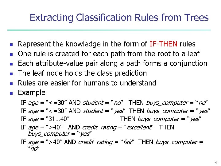
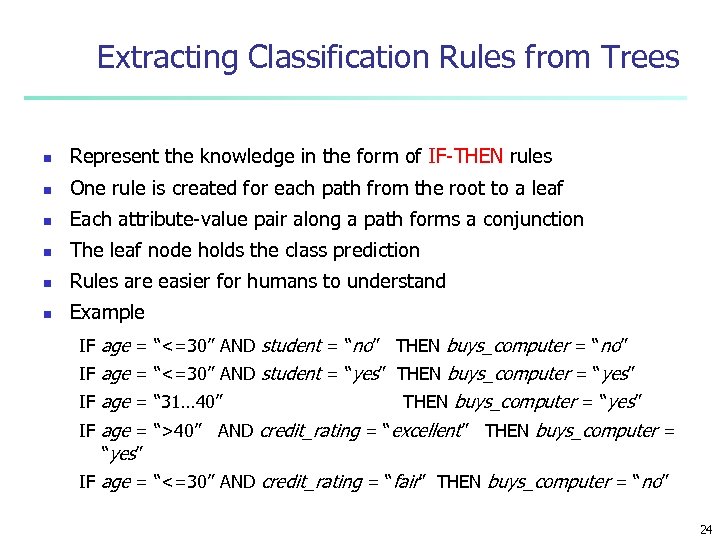Extracting Classification Rules from Trees n Represent the knowledge in the form of IF-THEN rules n One rule is created for each path from the root to a leaf n Each attribute-value pair along a path forms a conjunction n The leaf node holds the class prediction n Rules are easier for humans to understand n Example IF age = “<=30” AND student = “no” THEN buys_computer = “no” IF age = “<=30” AND student = “yes” THEN buys_computer = “yes” IF age = “ 31… 40” THEN buys_computer = “yes” IF age = “>40” AND credit_rating = “excellent” THEN buys_computer = “yes” IF age = “<=30” AND credit_rating = “fair” THEN buys_computer = “no” 24

Approaches to Determine the Final Tree Size n Separate training (2/3) and testing (1/3) sets n Use cross validation, e. g. , 10 -fold cross validation n Use all the data for training n n but apply a statistical test (e. g. , chi-square) to estimate whether expanding or pruning a node may improve the entire distribution Use minimum description length (MDL) principle n halting growth of the tree when the encoding is minimized 25

Enhancements to basic decision tree induction n Allow for continuous-valued attributes n n Dynamically define new discrete-valued attributes that partition the continuous attribute value into a discrete set of intervals Handle missing attribute values n n n Assign the most common value of the attribute Assign probability to each of the possible values Attribute construction n n Create new attributes based on existing ones that are sparsely represented This reduces fragmentation, repetition, and replication 26

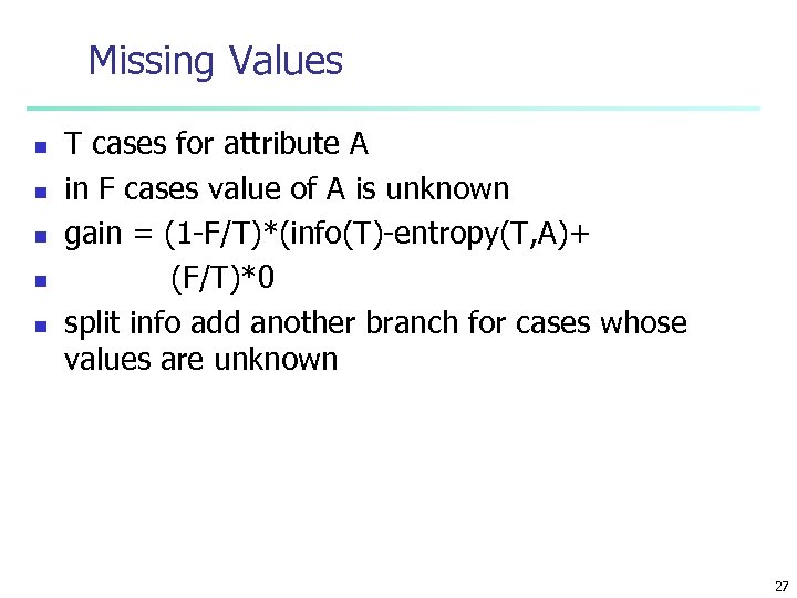Missing Values n n n T cases for attribute A in F cases value of A is unknown gain = (1 -F/T)*(info(T)-entropy(T, A)+ (F/T)*0 split info add another branch for cases whose values are unknown 27

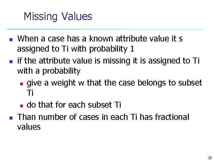Missing Values n n n When a case has a known attribute value it s assigned to Ti with probability 1 if the attribute value is missing it is assigned to Ti with a probability n give a weight w that the case belongs to subset Ti n do that for each subset Ti Than number of cases in each Ti has fractional values 28

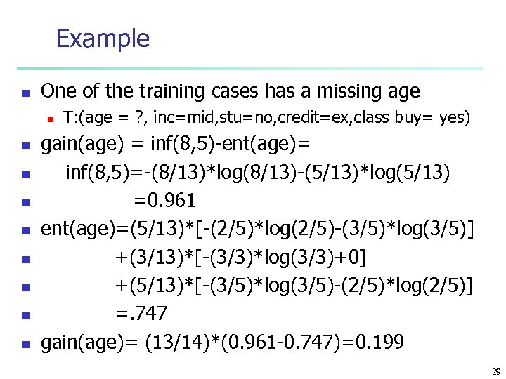Example n One of the training cases has a missing age n n n n n T: (age = ? , inc=mid, stu=no, credit=ex, class buy= yes) gain(age) = inf(8, 5)-ent(age)= inf(8, 5)=-(8/13)*log(8/13)-(5/13)*log(5/13) =0. 961 ent(age)=(5/13)*[-(2/5)*log(2/5)-(3/5)*log(3/5)] +(3/13)*[-(3/3)*log(3/3)+0] +(5/13)*[-(3/5)*log(3/5)-(2/5)*log(2/5)] =. 747 gain(age)= (13/14)*(0. 961 -0. 747)=0. 199 29

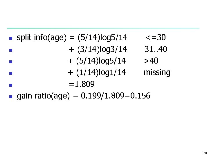n n n split info(age) = (5/14)log 5/14 <=30 + (3/14)log 3/14 31. . 40 + (5/14)log 5/14 >40 + (1/14)log 1/14 missing =1. 809 gain ratio(age) = 0. 199/1. 809=0. 156 30

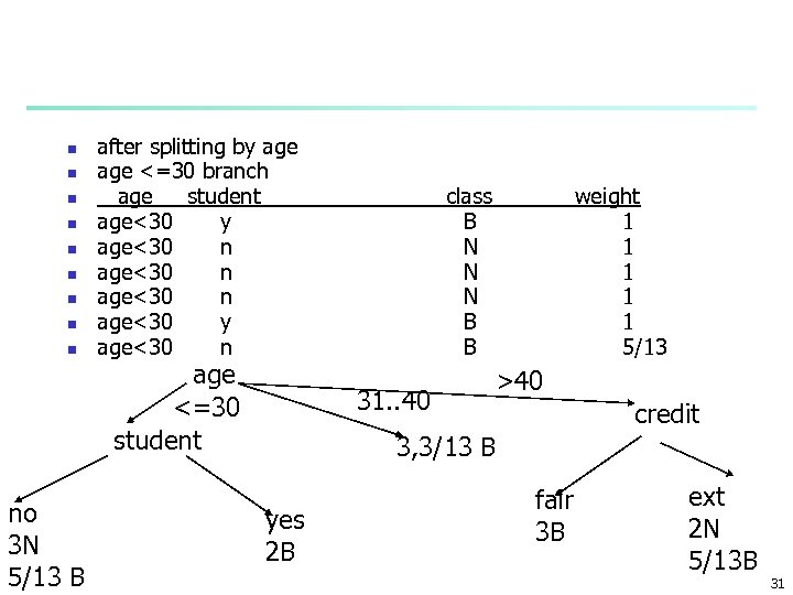n n no 3 N 5/13 B after splitting by age <=30 branch age student age<30 y age<30 n age<30 y age<30 n age <=30 student class B N N N B B 31. . 40 weight 1 1 1 5/13 >40 credit 3, 3/13 B yes 2 B fair 3 B ext 2 N 5/13 B 31

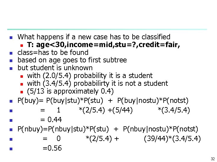n n n n n What happens if a new case has to be classified n T: age<30, income=mid, stu=? , credit=fair, class=has to be found based on age goes to first subtree but student is unknown n with (2. 0/5. 4) probability it is a student n with (3. 4/5. 4) probabilirty it is not a student n (5/13 is approximately 0. 4) P(buy)= P(buy|stu)*P(stu) + P(buy|nostu)*P(notst) = 1 *(2/5. 4) +(5/44) *(3. 4/5. 4) = 0. 44 P(nbuy)=P(nbuy|stu)*P(stu) + P(nbuy|nostu)*P(notst) = 0 *(2/5. 4) + (39/44)*(3. 4/5. 4) =0. 56 32

Continuous variables n n n Income is continuous make a binary split try all possible splitting points compute entropy and gain similarly but you can use income as a test variable in any subtree n there is still information in income not used perfectly 33

Avoid Overfitting in Classification n n Overfitting: An induced tree may overfit the training data n Too many branches, some may reflect anomalies due to noise or outliers n Poor accuracy for unseen samples Two approaches to avoid overfitting n Prepruning: Halt tree construction early—do not split a node if this would result in the goodness measure falling below a threshold n Difficult to choose an appropriate threshold n Postpruning: Remove branches from a “fully grown” tree—get a sequence of progressively pruned trees n Use a set of data different from the training data to decide which is the “best pruned tree” 34

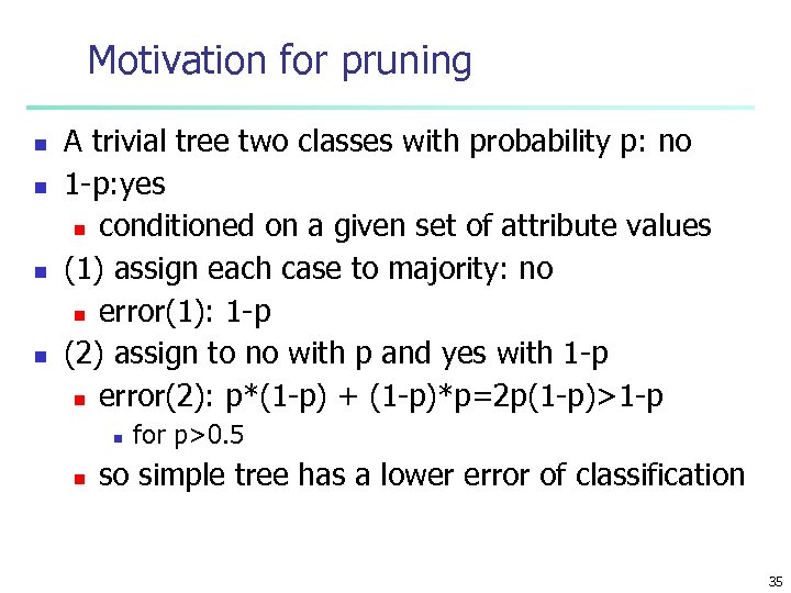Motivation for pruning n n A trivial tree two classes with probability p: no 1 -p: yes n conditioned on a given set of attribute values (1) assign each case to majority: no n error(1): 1 -p (2) assign to no with p and yes with 1 -p n error(2): p*(1 -p) + (1 -p)*p=2 p(1 -p)>1 -p n n for p>0. 5 so simple tree has a lower error of classification 35

n n If the error rate of a subtree is higher then the error obtained by replacing the tree with its most frequent leaf or branch n prune the subtree How to estimate the prediction error do not use training samples n pruning always increase error of the training sample estimate error based on test set n cost complexity or reduced error pruning 36

Pessimistic error estimates n n Based on training set only subtree covers N cases E cases missclasified error based on training set f=E/N n but this is not error n resemble it as a sample from population n estimate a upper bond on the population error based on the confidence limit Make a normal approximation to the binomial distribution 37

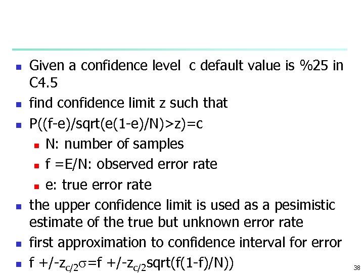n n n Given a confidence level c default value is %25 in C 4. 5 find confidence limit z such that P((f-e)/sqrt(e(1 -e)/N)>z)=c n N: number of samples n f =E/N: observed error rate n e: true error rate the upper confidence limit is used as a pesimistic estimate of the true but unknown error rate first approximation to confidence interval for error f +/-zc/2 =f +/-zc/2 sqrt(f(1 -f)/N)) 38

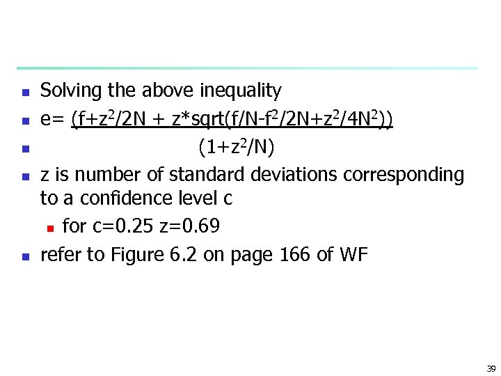n n n Solving the above inequality e= (f+z 2/2 N + z*sqrt(f/N-f 2/2 N+z 2/4 N 2)) (1+z 2/N) z is number of standard deviations corresponding to a confidence level c n for c=0. 25 z=0. 69 refer to Figure 6. 2 on page 166 of WF 39

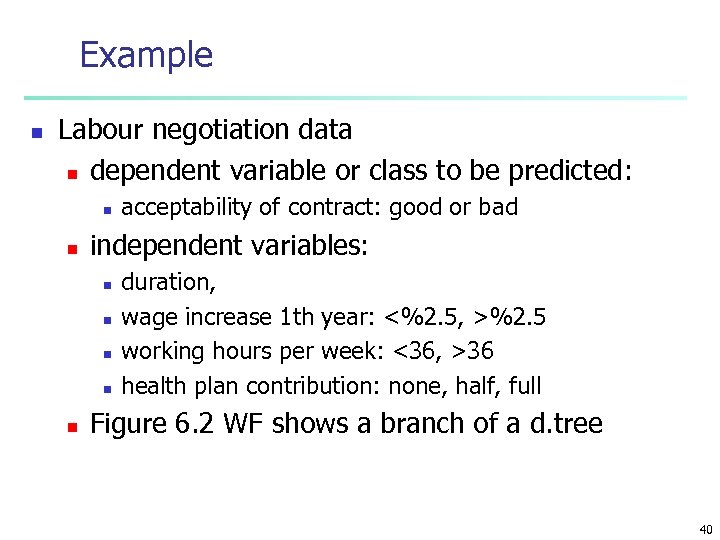Example n Labour negotiation data n dependent variable or class to be predicted: n n independent variables: n n n acceptability of contract: good or bad duration, wage increase 1 th year: <%2. 5, >%2. 5 working hours per week: <36, >36 health plan contribution: none, half, full Figure 6. 2 WF shows a branch of a d. tree 40

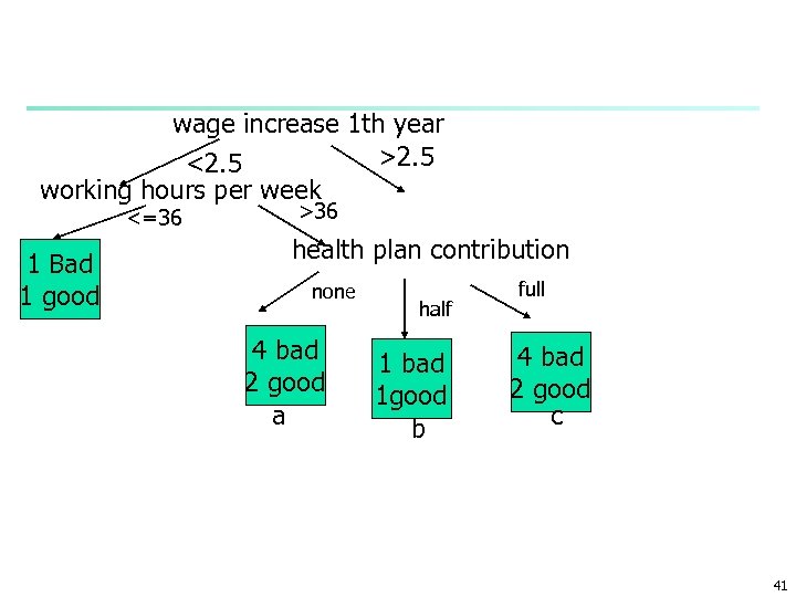wage increase 1 th year >2. 5 <2. 5 working hours per week <=36 1 Bad 1 good >36 health plan contribution none 4 bad 2 good a half 1 bad 1 good b full 4 bad 2 good c 41

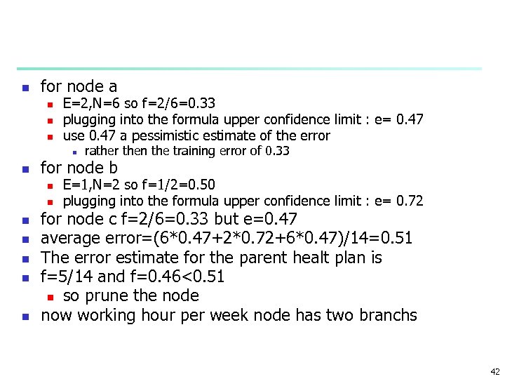n for node a n n n E=2, N=6 so f=2/6=0. 33 plugging into the formula upper confidence limit : e= 0. 47 use 0. 47 a pessimistic estimate of the error n n for node b n n n n rather then the training error of 0. 33 E=1, N=2 so f=1/2=0. 50 plugging into the formula upper confidence limit : e= 0. 72 for node c f=2/6=0. 33 but e=0. 47 average error=(6*0. 47+2*0. 72+6*0. 47)/14=0. 51 The error estimate for the parent healt plan is f=5/14 and f=0. 46<0. 51 n so prune the node now working hour per week node has two branchs 42

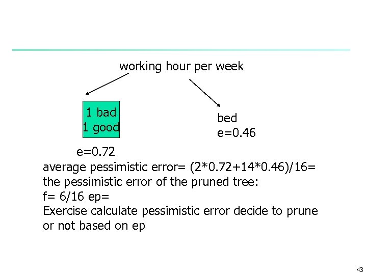working hour per week 1 bad 1 good bed e=0. 46 e=0. 72 average pessimistic error= (2*0. 72+14*0. 46)/16= the pessimistic error of the pruned tree: f= 6/16 ep= Exercise calculate pessimistic error decide to prune or not based on ep 43

Extracting Classification Rules from Trees n n n Represent the knowledge in the form of IF-THEN rules One rule is created for each path from the root to a leaf Each attribute-value pair along a path forms a conjunction The leaf node holds the class prediction Rules are easier for humans to understand Example age = “<=30” AND student = “no” THEN buys_computer = “no” age = “<=30” AND student = “yes” THEN buys_computer = “yes” age = “ 31… 40” THEN buys_computer = “yes” age = “>40” AND credit_rating = “excellent” THEN buys_computer = “yes” IF age = “>40” AND credit_rating = “fair” THEN buys_computer = “no” IF IF 44

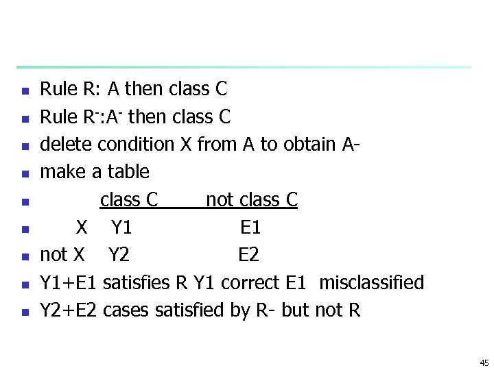n n n n n Rule R: A then class C Rule R-: A- then class C delete condition X from A to obtain Amake a table class C not class C X Y 1 E 1 not X Y 2 E 2 Y 1+E 1 satisfies R Y 1 correct E 1 misclassified Y 2+E 2 cases satisfied by R- but not R 45

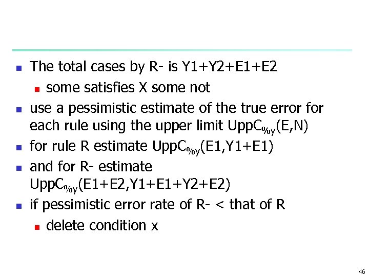n n n The total cases by R- is Y 1+Y 2+E 1+E 2 n some satisfies X some not use a pessimistic estimate of the true error for each rule using the upper limit Upp. C%y(E, N) for rule R estimate Upp. C%y(E 1, Y 1+E 1) and for R- estimate Upp. C%y(E 1+E 2, Y 1+E 1+Y 2+E 2) if pessimistic error rate of R- < that of R n delete condition x 46

n n n Suppose n conditions for a rule delete conditions one by one repeat n compare with the pessimistic error of the original rule n if min(R-)

Answer. Tree n Variables n n n n n measurement levels case weights frequency variables Growing methods Stopping rules Tree parameters n costs, prior probabilities, scores and profits Gain summary Accuracy of tree Cost-complexity pruning 48

Variables n n n Categorical Variables n nominal or ordinal Continuous Variables All grouping method accept all types of variables n QUEST requires that tatget variable be nominal Target and predictor variables n target variable (dependent variable) n predictor (independent variables) Case weight and frequency variables 49

Case weight and frequency variables n n n CASE WEIGHT VARIABLES unequal treatment to the cases Ex: direct marketing n n n all responders but %1 nonresponders(10, 000) n n n 10, 000 households respond and 1, 000 do not respond case weight 1 for responders and case weight 100 for nonresponders FREQUENCY VARIABLES n count of a record representing more than one individual 50

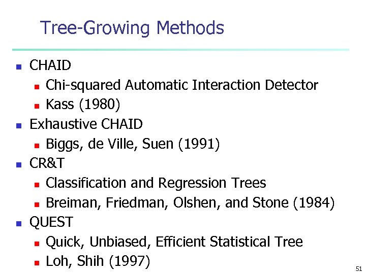Tree-Growing Methods n n CHAID n Chi-squared Automatic Interaction Detector n Kass (1980) Exhaustive CHAID n Biggs, de Ville, Suen (1991) CR&T n Classification and Regression Trees n Breiman, Friedman, Olshen, and Stone (1984) QUEST n Quick, Unbiased, Efficient Statistical Tree n Loh, Shih (1997) 51

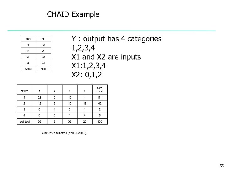
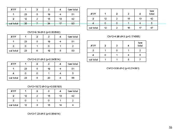
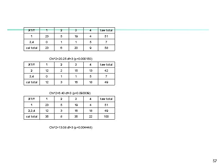
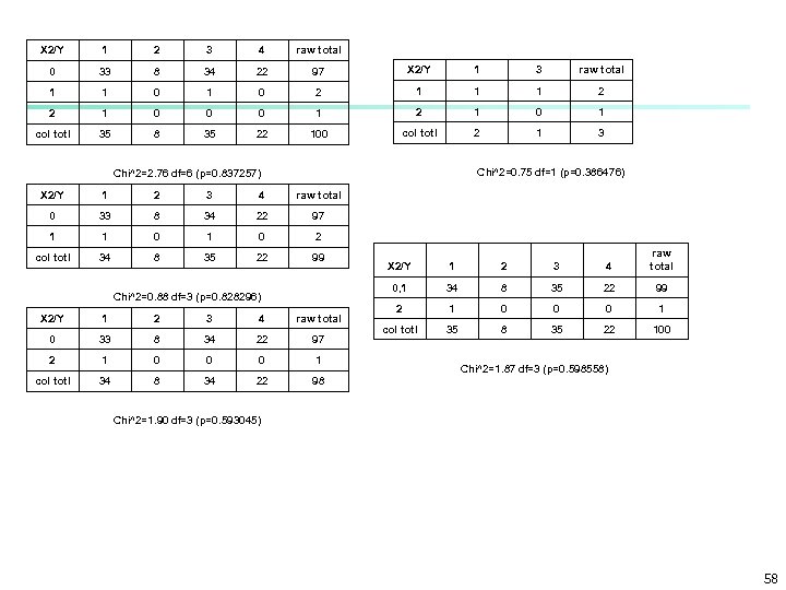
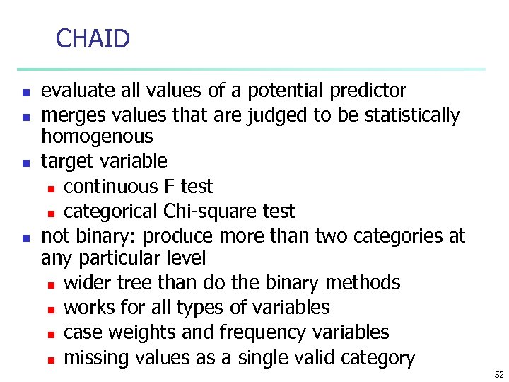CHAID n n evaluate all values of a potential predictor merges values that are judged to be statistically homogenous target variable n continuous F test n categorical Chi-square test not binary: produce more than two categories at any particular level n wider tree than do the binary methods n works for all types of variables n case weights and frequency variables n missing values as a single valid category 52

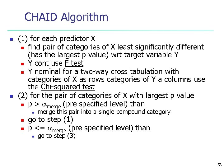CHAID Algorithm n n (1) for each predictor X n find pair of categories of X least significantly different (has the largest p value) wrt target variable Y n Y cont use F test n Y nominal for a two-way cross tabulation with categories of X as rows categories of Y a columns use the Chi-squared test (2) for the pair of categories of X with largest p value n p > merge (pre specified level) than n merge this pair into a single compound category go to step (1) p <= merge (pre specified level) than n go to step (3) 53

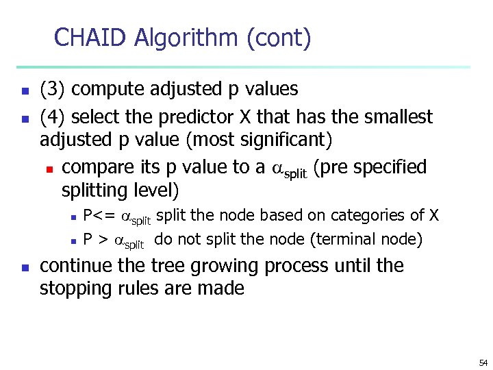CHAID Algorithm (cont) n n (3) compute adjusted p values (4) select the predictor X that has the smallest adjusted p value (most significant) n compare its p value to a split (pre specified splitting level) n n n P<= split the node based on categories of X P > split do not split the node (terminal node) continue the tree growing process until the stopping rules are made 54

CHAID Example cat 1 35 2 8 3 35 4 22 total Y : output has 4 categories 1, 2, 3, 4 X 1 and X 2 are inputs X 1: 1, 2, 3, 4 X 2: 0, 1, 2 # 100 X 1/Y 1 2 3 4 raw total 1 23 5 19 4 51 2 12 2 15 13 42 3 0 1 2 4 0 0 1 4 5 col totl 35 8 35 22 100 Chi^2=25. 63 df=9 (p=0. 002342) 55

X 1/Y 1 2 3 4 taw total 1 23 5 19 4 51 X 1/Y 1 2 3 4 taw total 2 12 2 15 13 42 cal total 35 7 34 17 93 4 0 0 1 4 5 cal total 12 2 16 17 47 Chi^2=9. 19 df=3 (p=0. 002682) Chi^2=4. 96 df=3 (p=0. 174565) X 1/Y 1 2 3 4 taw total 1 23 5 19 4 51 3 0 1 2 X 1/Y 2 3 4 taw total cal total 23 6 19 5 53 3 1 0 1 2 4 0 1 4 5 cal total 1 1 5 7 Chi^2=8. 01 df=3 (p=0. 045614) X 1/Y 1 2 3 4 taw total 1 23 5 19 4 51 4 0 0 1 4 5 cal total 23 5 20 8 56 Chi^2=3. 08 df=2 (p=0. 214381) Chi^2=19. 72 df=3 (p=0. 000193) X 1/Y 1 2 3 4 taw total 2 12 2 15 13 42 3 0 1 2 cal total 12 3 15 14 4 Chi^2=7. 23 df=3 (p=0. 064814) 56

X 1/Y 1 2 3 4 taw total 1 23 5 19 4 51 3, 4 0 1 1 5 7 cal total 23 6 20 9 58 Chi^2=20. 25 df=3 (p=0. 000150) X 1/Y 1 2 3 4 taw total 2 12 2 15 13 42 3, 4 0 1 1 5 7 cal total 12 3 16 18 49 Chi^2=6. 40 df=3 (p=0. 093339) X 1/Y 1 2 3 4 taw total 1 23 5 19 4 51 2, 3, 4 12 3 16 18 49 cal total 35 8 35 22 100 Chi^2=13. 08 df=3 (p=0. 004448) 57

X 2/Y 1 2 3 4 raw total 0 33 8 34 22 97 X 2/Y 1 3 raw total 1 1 0 2 1 1 1 2 2 1 0 0 0 1 2 1 0 1 col totl 35 8 35 22 100 col totl 2 1 3 Chi^2=0. 75 df=1 (p=0. 386476) Chi^2=2. 76 df=6 (p=0. 837257) X 2/Y 1 2 3 4 raw total 0 33 8 34 22 97 1 1 0 2 col totl 34 8 35 22 99 X 2/Y 1 2 3 4 raw total 0 33 8 34 22 97 2 1 0 0 0 1 col totl 34 8 34 22 1 2 3 4 raw total 0, 1 Chi^2=0. 88 df=3 (p=0. 828296) X 2/Y 34 8 35 22 99 2 1 0 0 0 1 col totl 35 8 35 22 100 98 Chi^2=1. 87 df=3 (p=0. 598558) Chi^2=1. 90 df=3 (p=0. 593045) 58

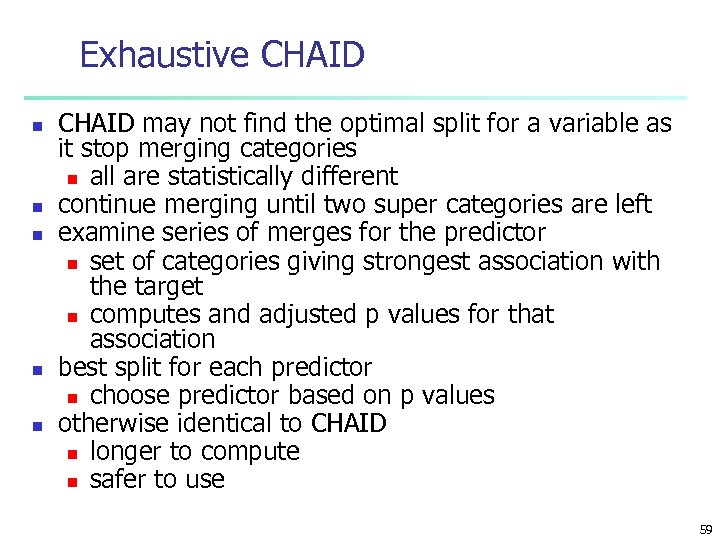Exhaustive CHAID n n n CHAID may not find the optimal split for a variable as it stop merging categories n all are statistically different continue merging until two super categories are left examine series of merges for the predictor n set of categories giving strongest association with the target n computes and adjusted p values for that association best split for each predictor n choose predictor based on p values otherwise identical to CHAID n longer to compute n safer to use 59

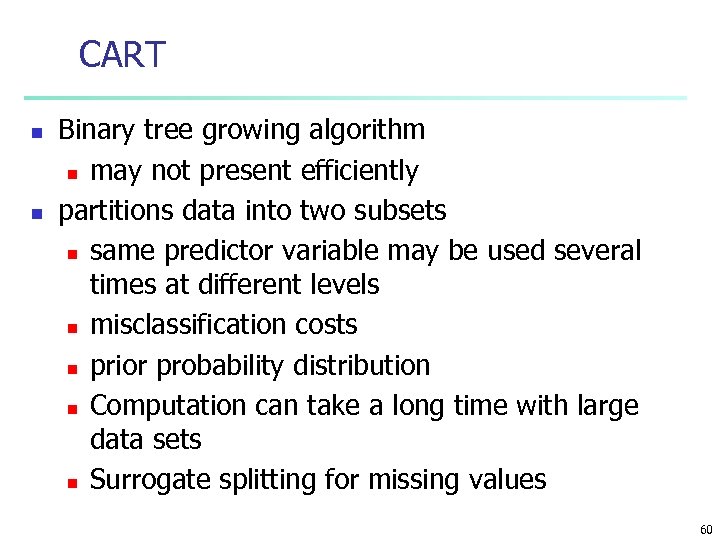CART n n Binary tree growing algorithm n may not present efficiently partitions data into two subsets n same predictor variable may be used several times at different levels n misclassification costs n prior probability distribution n Computation can take a long time with large data sets n Surrogate splitting for missing values 60

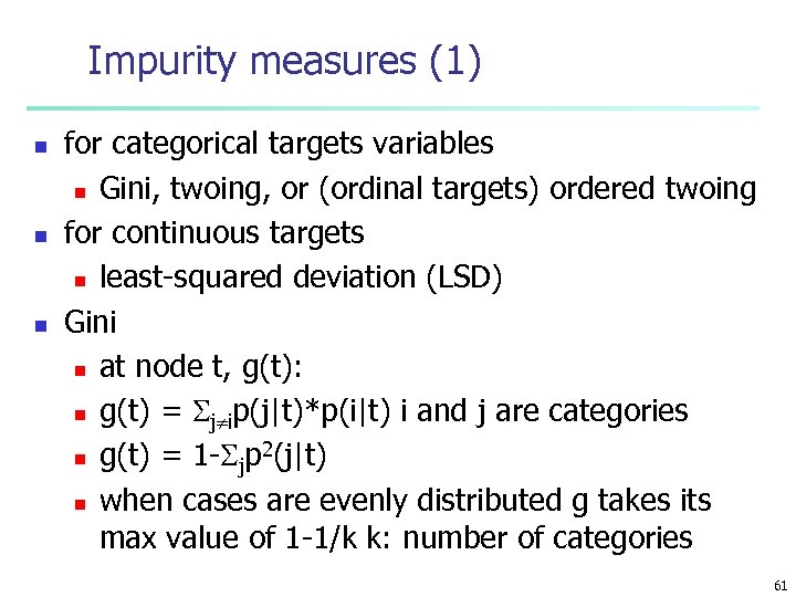Impurity measures (1) n n n for categorical targets variables n Gini, twoing, or (ordinal targets) ordered twoing for continuous targets n least-squared deviation (LSD) Gini n at node t, g(t): n g(t) = j ip(j|t)*p(i|t) i and j are categories 2 n g(t) = 1 - jp (j|t) n when cases are evenly distributed g takes its max value of 1 -1/k k: number of categories 61

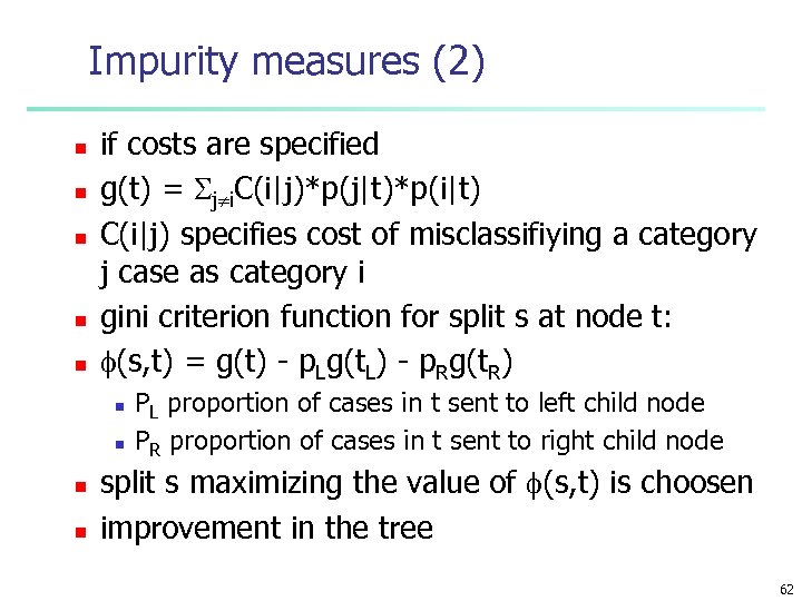Impurity measures (2) n n n if costs are specified g(t) = j i. C(i|j)*p(j|t)*p(i|t) C(i|j) specifies cost of misclassifiying a category j case as category i gini criterion function for split s at node t: (s, t) = g(t) - p. Lg(t. L) - p. Rg(t. R) n n PL proportion of cases in t sent to left child node PR proportion of cases in t sent to right child node split s maximizing the value of (s, t) is choosen improvement in the tree 62

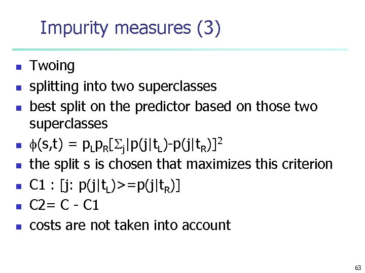Impurity measures (3) n n n n Twoing splitting into two superclasses best split on the predictor based on those two superclasses (s, t) = p. Lp. R[ j|p(j|t. L)-p(j|t. R)]2 the split s is chosen that maximizes this criterion C 1 : [j: p(j|t. L)>=p(j|t. R)] C 2= C - C 1 costs are not taken into account 63

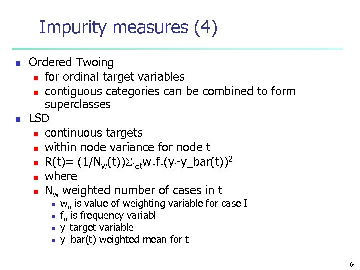Impurity measures (4) n n Ordered Twoing n for ordinal target variables n contiguous categories can be combined to form superclasses LSD n continuous targets n within node variance for node t 2 n R(t)= (1/Nw(t)) i twnfn(yi-y_bar(t)) n where n Nw weighted number of cases in t n n wn is value of weighting variable for case I fn is frequency variabl yi target variable y_bar(t) weighted mean for t 64

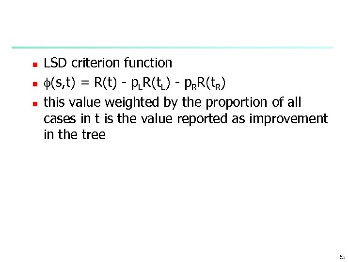n n n LSD criterion function (s, t) = R(t) - p. LR(t. L) - p. RR(t. R) this value weighted by the proportion of all cases in t is the value reported as improvement in the tree 65

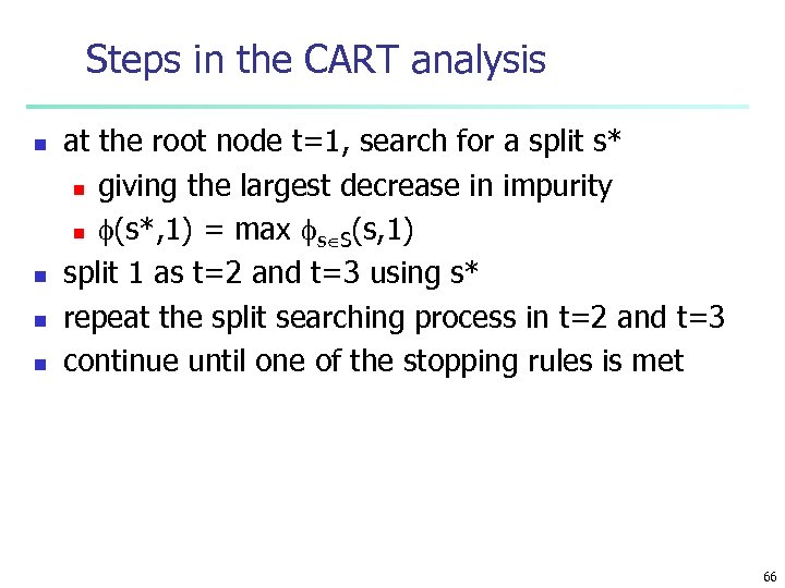Steps in the CART analysis n n at the root node t=1, search for a split s* n giving the largest decrease in impurity n (s*, 1) = max s S(s, 1) split 1 as t=2 and t=3 using s* repeat the split searching process in t=2 and t=3 continue until one of the stopping rules is met 66

Stoping rules n n n all cases have identical values for all predictors the node becomes pure; all cases have the same value of the target variable the depth of the tree has reached its prespecified maximum value the number of cases in a node less than a prespecified minimum parent node size split at node results in producing a child node with cases less than a prespecified min child node size for CART only: max decrease in impurity is less than a prespecified value 67

QUEST n n variable selection and split point selection separately computationally efficient than CART 68

Classification in Large Databases n n n Classification—a classical problem extensively studied by statisticians and machine learning researchers Scalability: Classifying data sets with millions of examples and hundreds of attributes with reasonable speed Why decision tree induction in data mining? n relatively faster learning speed (than other classification methods) n convertible to simple and easy to understand classification rules n can use SQL queries for accessing databases n comparable classification accuracy with other methods 69

Scalable Decision Tree Induction Methods in Data Mining Studies n n SLIQ (EDBT’ 96 — Mehta et al. ) n builds an index for each attribute and only class list and the current attribute list reside in memory SPRINT (VLDB’ 96 — J. Shafer et al. ) n constructs an attribute list data structure PUBLIC (VLDB’ 98 — Rastogi & Shim) n integrates tree splitting and tree pruning: stop growing the tree earlier Rain. Forest (VLDB’ 98 — Gehrke, Ramakrishnan & Ganti) n separates the scalability aspects from the criteria that determine the quality of the tree n builds an AVC-list (attribute, value, class label) 70

Data Cube-Based Decision-Tree Induction n n Integration of generalization with decision-tree induction (Kamber et al’ 97). Classification at primitive concept levels n n E. g. , precise temperature, humidity, outlook, etc. Low-level concepts, scattered classes, bushy classification-trees Semantic interpretation problems. Cube-based multi-level classification n Relevance analysis at multi-levels. n Information-gain analysis with dimension + level. 71

Chapter 7. Classification and Prediction n n What is classification? What is prediction? Issues regarding classification and prediction Classification by decision tree induction Bayesian Classification by Neural Networks Classification by Support Vector Machines (SVM) Classification based on concepts from association rule mining Other Classification Methods Prediction Classification accuracy Summary 72

Bayesian Classification: Why? n n Probabilistic learning: Calculate explicit probabilities for hypothesis, among the most practical approaches to certain types of learning problems Incremental: Each training example can incrementally increase/decrease the probability that a hypothesis is correct. Prior knowledge can be combined with observed data. Probabilistic prediction: Predict multiple hypotheses, weighted by their probabilities Standard: Even when Bayesian methods are computationally intractable, they can provide a standard of optimal decision making against which other methods can be measured 73

Bayesian Theorem: Basics n n n Let X be a data sample whose class label is unknown Let H be a hypothesis that X belongs to class C For classification problems, determine P(H/X): the probability that the hypothesis holds given the observed data sample X P(H): prior probability of hypothesis H (i. e. the initial probability before we observe any data, reflects the background knowledge) P(X): probability that sample data is observed P(X|H) : probability of observing the sample X, given that the hypothesis holds 74

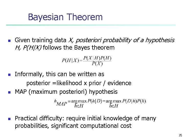Bayesian Theorem n n Given training data X, posteriori probability of a hypothesis H, P(H|X) follows the Bayes theorem Informally, this can be written as posterior =likelihood x prior / evidence MAP (maximum posteriori) hypothesis Practical difficulty: require initial knowledge of many probabilities, significant computational cost 75

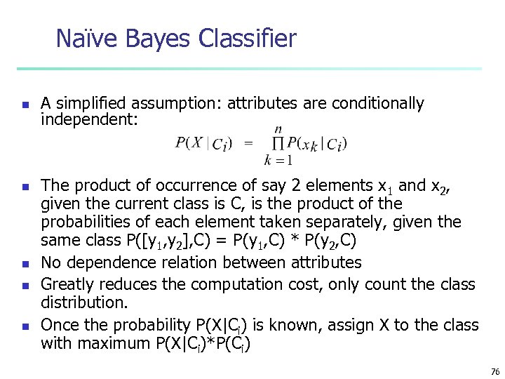Naïve Bayes Classifier n n n A simplified assumption: attributes are conditionally independent: The product of occurrence of say 2 elements x 1 and x 2, given the current class is C, is the product of the probabilities of each element taken separately, given the same class P([y 1, y 2], C) = P(y 1, C) * P(y 2, C) No dependence relation between attributes Greatly reduces the computation cost, only count the class distribution. Once the probability P(X|Ci) is known, assign X to the class with maximum P(X|Ci)*P(Ci) 76

Example n n n H X is an apple P(H) priori probability that X is an apple X observed data round and red P(H/X) probability that X is an apple given that we observe that it is red and round P(X/H) posteriori probability that a data is red and round given that it is an apple P(X) priori probabilility that it is red and round 77

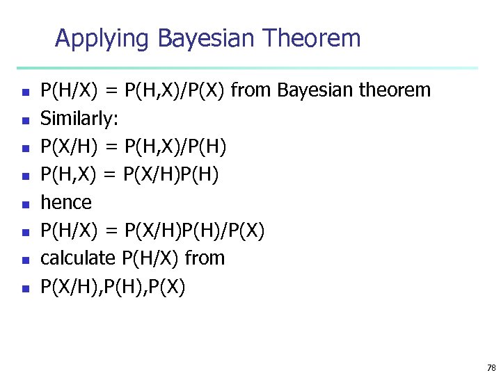Applying Bayesian Theorem n n n n P(H/X) = P(H, X)/P(X) from Bayesian theorem Similarly: P(X/H) = P(H, X)/P(H) P(H, X) = P(X/H)P(H) hence P(H/X) = P(X/H)P(H)/P(X) calculate P(H/X) from P(X/H), P(X) 78

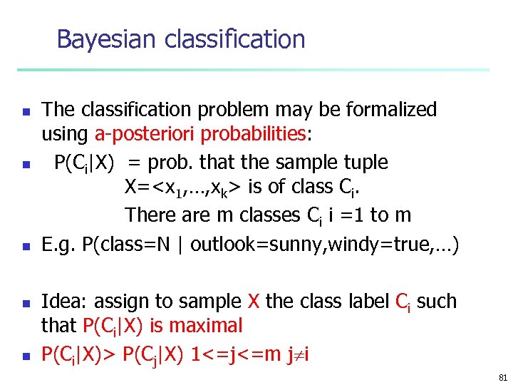Bayesian classification n n The classification problem may be formalized using a-posteriori probabilities: P(Ci|X) = prob. that the sample tuple X= is of class Ci. There are m classes Ci i =1 to m E. g. P(class=N | outlook=sunny, windy=true, …) Idea: assign to sample X the class label Ci such that P(Ci|X) is maximal P(Ci|X)> P(Cj|X) 1<=j<=m j i 81

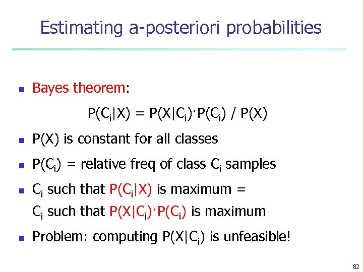Estimating a-posteriori probabilities n Bayes theorem: P(Ci|X) = P(X|Ci)·P(Ci) / P(X) n P(X) is constant for all classes n P(Ci) = relative freq of class Ci samples n Ci such that P(Ci|X) is maximum = Ci such that P(X|Ci)·P(Ci) is maximum n Problem: computing P(X|Ci) is unfeasible! 82

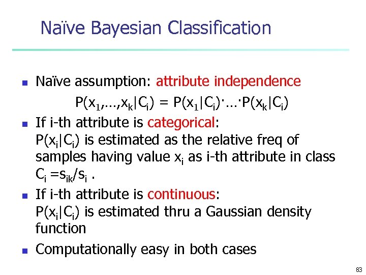Naïve Bayesian Classification n n Naïve assumption: attribute independence P(x 1, …, xk|Ci) = P(x 1|Ci)·…·P(xk|Ci) If i-th attribute is categorical: P(xi|Ci) is estimated as the relative freq of samples having value xi as i-th attribute in class Ci =sik/si. If i-th attribute is continuous: P(xi|Ci) is estimated thru a Gaussian density function Computationally easy in both cases 83

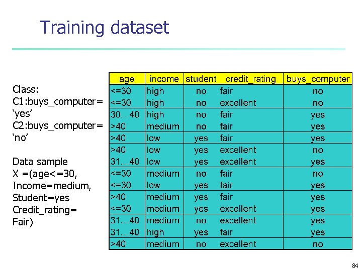Training dataset Class: C 1: buys_computer= ‘yes’ C 2: buys_computer= ‘no’ Data sample X =(age<=30, Income=medium, Student=yes Credit_rating= Fair) 84

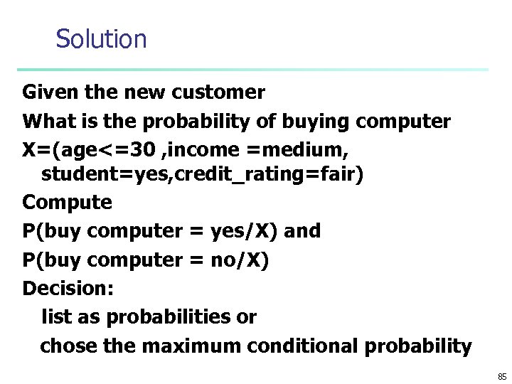Solution Given the new customer What is the probability of buying computer X=(age<=30 , income =medium, student=yes, credit_rating=fair) Compute P(buy computer = yes/X) and P(buy computer = no/X) Decision: list as probabilities or chose the maximum conditional probability 85

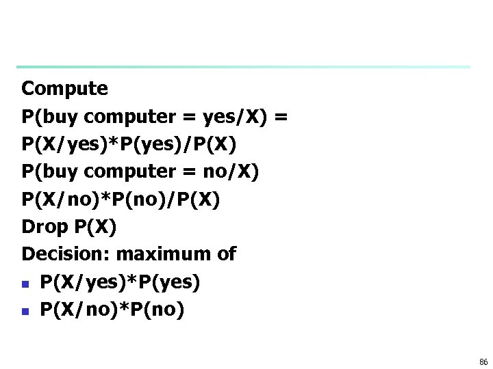Compute P(buy computer = yes/X) = P(X/yes)*P(yes)/P(X) P(buy computer = no/X) P(X/no)*P(no)/P(X) Drop P(X) Decision: maximum of n P(X/yes)*P(yes) n P(X/no)*P(no) 86

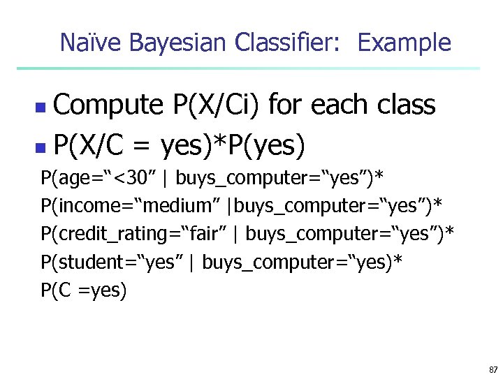Naïve Bayesian Classifier: Example Compute P(X/Ci) for each class n P(X/C = yes)*P(yes) n P(age=“<30” | buys_computer=“yes”)* P(income=“medium” |buys_computer=“yes”)* P(credit_rating=“fair” | buys_computer=“yes”)* P(student=“yes” | buys_computer=“yes)* P(C =yes) 87

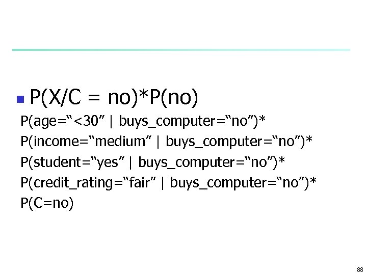n P(X/C = no)*P(no) P(age=“<30” | buys_computer=“no”)* P(income=“medium” | buys_computer=“no”)* P(student=“yes” | buys_computer=“no”)* P(credit_rating=“fair” | buys_computer=“no”)* P(C=no) 88

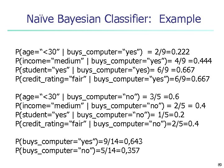Naïve Bayesian Classifier: Example P(age=“<30” | buys_computer=“yes”) = 2/9=0. 222 P(income=“medium” | buys_computer=“yes”)= 4/9 =0. 444 P(student=“yes” | buys_computer=“yes)= 6/9 =0. 667 P(credit_rating=“fair” | buys_computer=“yes”)=6/9=0. 667 P(age=“<30” | buys_computer=“no”) = 3/5 =0. 6 P(income=“medium” | buys_computer=“no”) = 2/5 = 0. 4 P(student=“yes” | buys_computer=“no”)= 1/5=0. 2 P(credit_rating=“fair” | buys_computer=“no”)=2/5=0. 4 P(buys_computer=“yes”)=9/14=0, 643 P(buys_computer=“no”)=5/14=0, 357 89

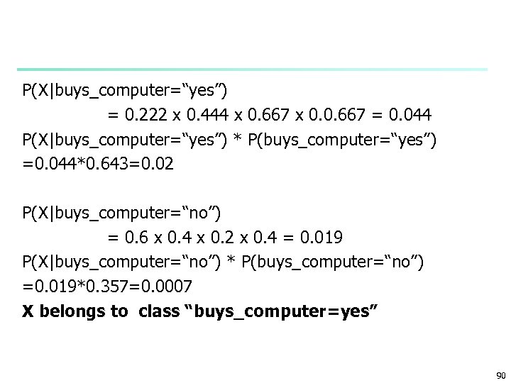P(X|buys_computer=“yes”) = 0. 222 x 0. 444 x 0. 667 x 0. 0. 667 = 0. 044 P(X|buys_computer=“yes”) * P(buys_computer=“yes”) =0. 044*0. 643=0. 02 P(X|buys_computer=“no”) = 0. 6 x 0. 4 x 0. 2 x 0. 4 = 0. 019 P(X|buys_computer=“no”) * P(buys_computer=“no”) =0. 019*0. 357=0. 0007 X belongs to class “buys_computer=yes” 90

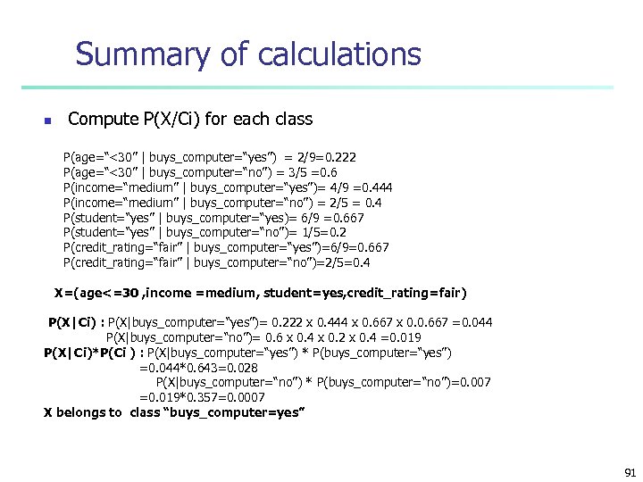Summary of calculations n Compute P(X/Ci) for each class P(age=“<30” | buys_computer=“yes”) = 2/9=0. 222 P(age=“<30” | buys_computer=“no”) = 3/5 =0. 6 P(income=“medium” | buys_computer=“yes”)= 4/9 =0. 444 P(income=“medium” | buys_computer=“no”) = 2/5 = 0. 4 P(student=“yes” | buys_computer=“yes)= 6/9 =0. 667 P(student=“yes” | buys_computer=“no”)= 1/5=0. 2 P(credit_rating=“fair” | buys_computer=“yes”)=6/9=0. 667 P(credit_rating=“fair” | buys_computer=“no”)=2/5=0. 4 X=(age<=30 , income =medium, student=yes, credit_rating=fair) P(X|Ci) : P(X|buys_computer=“yes”)= 0. 222 x 0. 444 x 0. 667 x 0. 0. 667 =0. 044 P(X|buys_computer=“no”)= 0. 6 x 0. 4 x 0. 2 x 0. 4 =0. 019 P(X|Ci)*P(Ci ) : P(X|buys_computer=“yes”) * P(buys_computer=“yes”) =0. 044*0. 643=0. 028 P(X|buys_computer=“no”) * P(buys_computer=“no”)=0. 007 =0. 019*0. 357=0. 0007 X belongs to class “buys_computer=yes” 91

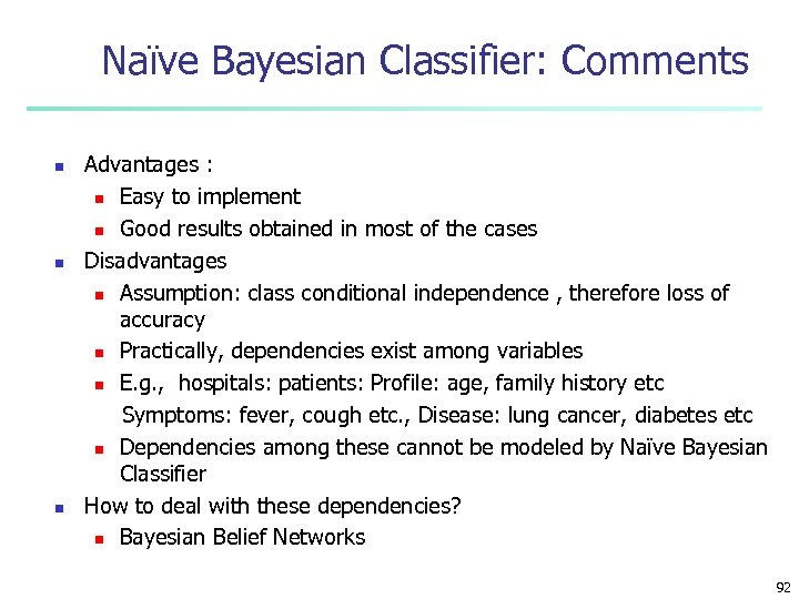Naïve Bayesian Classifier: Comments n n n Advantages : n Easy to implement n Good results obtained in most of the cases Disadvantages n Assumption: class conditional independence , therefore loss of accuracy n Practically, dependencies exist among variables n E. g. , hospitals: patients: Profile: age, family history etc Symptoms: fever, cough etc. , Disease: lung cancer, diabetes etc n Dependencies among these cannot be modeled by Naïve Bayesian Classifier How to deal with these dependencies? n Bayesian Belief Networks 92

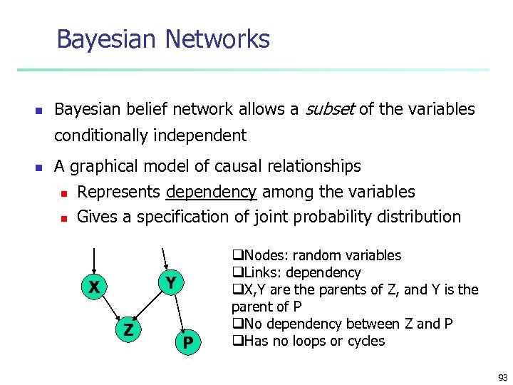Bayesian Networks n Bayesian belief network allows a subset of the variables conditionally independent n A graphical model of causal relationships n n Represents dependency among the variables Gives a specification of joint probability distribution Y X Z P q. Nodes: random variables q. Links: dependency q. X, Y are the parents of Z, and Y is the parent of P q. No dependency between Z and P q. Has no loops or cycles 93

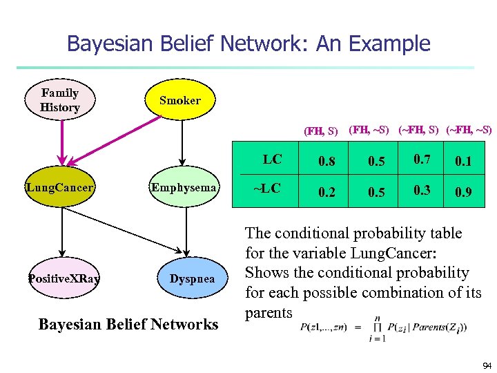Bayesian Belief Network: An Example Family History Smoker (FH, S) (FH, ~S) (~FH, ~S) LC Lung. Cancer Positive. XRay Emphysema Dyspnea Bayesian Belief Networks 0. 8 0. 5 0. 7 0. 1 ~LC 0. 2 0. 5 0. 3 0. 9 The conditional probability table for the variable Lung. Cancer: Shows the conditional probability for each possible combination of its parents 94

Learning Bayesian Networks n n Several cases n Given both the network structure and all variables observable: learn only the CPTs n Network structure known, some hidden variables: method of gradient descent, analogous to neural network learning n Network structure unknown, all variables observable: search through the model space to reconstruct graph topology n Unknown structure, all hidden variables: no good algorithms known for this purpose D. Heckerman, Bayesian networks for data mining 95