Data Quality and Data Cleaning An Overview Theodore

Data Quality and Data Cleaning: An Overview Theodore Johnson johnsont@research. att. com AT&T Labs – Research (Lecture notes for CS 541, 02/12/2004)

Based on: • Recent book Exploratory Data Mining and Data Quality Dasu and Johnson (Wiley, 2004) • SIGMOD 2003 tutorial.

Tutorial Focus • What research is relevant to Data Quality? – DQ is pervasive and expensive. It is an important problem. – But the problems are so messy and unstructured that research seems irrelevant. • This tutorial will try to structure the problem to make research directions more clear. • Overview – Data quality process • Where do problems come from • How can they be resolved – Disciplines • • Management Statistics Database Metadata

Overview • • • The meaning of data quality (1) The data quality continuum The meaning of data quality (2) Data quality metrics Technical tools – – Management Statistical Database Metadata • Case Study • Research directions

The Meaning of Data Quality (1)

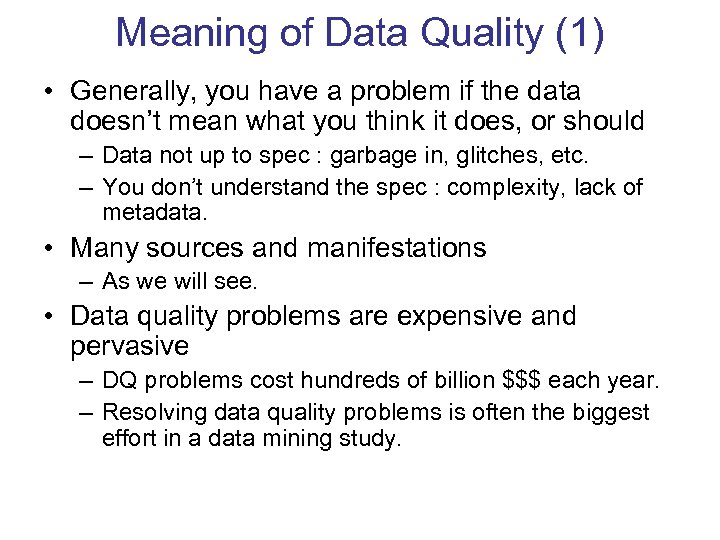Meaning of Data Quality (1) • Generally, you have a problem if the data doesn’t mean what you think it does, or should – Data not up to spec : garbage in, glitches, etc. – You don’t understand the spec : complexity, lack of metadata. • Many sources and manifestations – As we will see. • Data quality problems are expensive and pervasive – DQ problems cost hundreds of billion $$$ each year. – Resolving data quality problems is often the biggest effort in a data mining study.

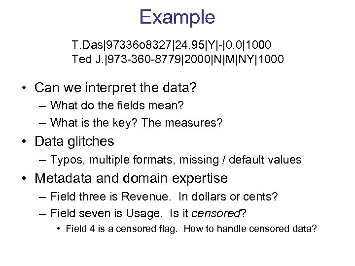Example T. Das|97336 o 8327|24. 95|Y|-|0. 0|1000 Ted J. |973 -360 -8779|2000|N|M|NY|1000 • Can we interpret the data? – What do the fields mean? – What is the key? The measures? • Data glitches – Typos, multiple formats, missing / default values • Metadata and domain expertise – Field three is Revenue. In dollars or cents? – Field seven is Usage. Is it censored? • Field 4 is a censored flag. How to handle censored data?

Data Glitches • Systemic changes to data which are external to the recorded process. – Changes in data layout / data types • Integer becomes string, fields swap positions, etc. – Changes in scale / format • Dollars vs. euros – Temporary reversion to defaults • Failure of a processing step – Missing and default values • Application programs do not handle NULL values well … – Gaps in time series • Especially when records represent incremental changes.

Conventional Definition of Data Quality • Accuracy – The data was recorded correctly. • Completeness – All relevant data was recorded. • Uniqueness – Entities are recorded once. • Timeliness – The data is kept up to date. • Special problems in federated data: time consistency. • Consistency – The data agrees with itself.

Problems … • Unmeasurable – Accuracy and completeness are extremely difficult, perhaps impossible to measure. • Context independent – No accounting for what is important. E. g. , if you are computing aggregates, you can tolerate a lot of inaccuracy. • Incomplete – What about interpretability, accessibility, metadata, analysis, etc. • Vague – The conventional definitions provide no guidance towards practical improvements of the data.

Finding a modern definition • We need a definition of data quality which – Reflects the use of the data – Leads to improvements in processes – Is measurable (we can define metrics) • First, we need a better understanding of how and where data quality problems occur – The data quality continuum

The Data Quality Continuum

The Data Quality Continuum • Data and information is not static, it flows in a data collection and usage process – – – Data gathering Data delivery Data storage Data integration Data retrieval Data mining/analysis

Data Gathering • How does the data enter the system? • Sources of problems: – Manual entry – No uniform standards for content and formats – Parallel data entry (duplicates) – Approximations, surrogates – SW/HW constraints – Measurement errors.

Solutions • Potential Solutions: – Preemptive: • Process architecture (build in integrity checks) • Process management (reward accurate data entry, data sharing, data stewards) – Retrospective: • Cleaning focus (duplicate removal, merge/purge, name & address matching, field value standardization) • Diagnostic focus (automated detection of glitches).

Data Delivery • Destroying or mutilating information by inappropriate pre-processing – Inappropriate aggregation – Nulls converted to default values • Loss of data: – Buffer overflows – Transmission problems – No checks

Solutions • Build reliable transmission protocols – Use a relay server • Verification – Checksums, verification parser – Do the uploaded files fit an expected pattern? • Relationships – Are there dependencies between data streams and processing steps • Interface agreements – Data quality commitment from the data stream supplier.

Data Storage • You get a data set. What do you do with it? • Problems in physical storage – Can be an issue, but terabytes are cheap. • Problems in logical storage (ER relations) – Poor metadata. • Data feeds are often derived from application programs or legacy data sources. What does it mean? – Inappropriate data models. • Missing timestamps, incorrect normalization, etc. – Ad-hoc modifications. • Structure the data to fit the GUI. – Hardware / software constraints. • Data transmission via Excel spreadsheets, Y 2 K

Solutions • Metadata – Document and publish data specifications. • Planning – Assume that everything bad will happen. – Can be very difficult. • Data exploration – Use data browsing and data mining tools to examine the data. • Does it meet the specifications you assumed? • Has something changed?

Data Integration • Combine data sets (acquisitions, across departments). • Common source of problems – Heterogenous data : no common key, different field formats • Approximate matching – Different definitions • What is a customer: an account, an individual, a family, … – Time synchronization • Does the data relate to the same time periods? Are the time windows compatible? – Legacy data • IMS, spreadsheets, ad-hoc structures – Sociological factors • Reluctance to share – loss of power.

Solutions • Commercial Tools – Significant body of research in data integration – Many tools for address matching, schema mapping are available. • Data browsing and exploration – Many hidden problems and meanings : must extract metadata. – View before and after results : did the integration go the way you thought?

Data Retrieval • Exported data sets are often a view of the actual data. Problems occur because: – Source data not properly understood. – Need for derived data not understood. – Just plain mistakes. • Inner join vs. outer join • Understanding NULL values • Computational constraints – E. g. , too expensive to give a full history, we’ll supply a snapshot. • Incompatibility – Ebcdic?

Data Mining and Analysis • What are you doing with all this data anyway? • Problems in the analysis. – Scale and performance – Confidence bounds? – Black boxes and dart boards • “fire your Statisticians” – Attachment to models – Insufficient domain expertise – Casual empiricism

Solutions • Data exploration – Determine which models and techniques are appropriate, find data bugs, develop domain expertise. • Continuous analysis – Are the results stable? How do they change? • Accountability – Make the analysis part of the feedback loop.

The Meaning of Data Quality (2)

Meaning of Data Quality (2) • There are many types of data, which have different uses and typical quality problems – – – – Federated data High dimensional data Descriptive data Longitudinal data Streaming data Web (scraped) data Numeric vs. categorical vs. text data

Meaning of Data Quality (2) • There are many uses of data – Operations – Aggregate analysis – Customer relations … • Data Interpretation : the data is useless if we don’t know all of the rules behind the data. • Data Suitability : Can you get the answer from the available data – Use of proxy data – Relevant data is missing

Data Quality Constraints • Many data quality problems can be captured by static constraints based on the schema. – Nulls not allowed, field domains, foreign key constraints, etc. • Many others are due to problems in workflow, and can be captured by dynamic constraints – E. g. , orders above $200 are processed by Biller 2 • The constraints follow an 80 -20 rule – A few constraints capture most cases, thousands of constraints to capture the last few cases. • Constraints are measurable. Data Quality Metrics?

Data Quality Metrics

Data Quality Metrics • We want a measurable quantity – Indicates what is wrong and how to improve – Realize that DQ is a messy problem, no set of numbers will be perfect • Types of metrics – Static vs. dynamic constraints – Operational vs. diagnostic • Metrics should be directionally correct with an improvement in use of the data. • A very large number metrics are possible – Choose the most important ones.

Examples of Data Quality Metrics • Conformance to schema – Evaluate constraints on a snapshot. • Conformance to business rules – Evaluate constraints on changes in the database. • Accuracy – Perform inventory (expensive), or use proxy (track complaints). Audit samples? • • Accessibility Interpretability Glitches in analysis Successful completion of end-to-end process

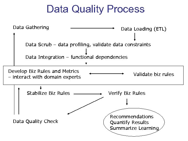Data Quality Process Data Gathering Data Loading (ETL) Data Scrub – data profiling, validate data constraints Data Integration – functional dependencies Develop Biz Rules and Metrics – interact with domain experts Stabilize Biz Rules Data Quality Check Validate biz rules Verify Biz Rules Recommendations Quantify Results Summarize Learning

Technical Tools

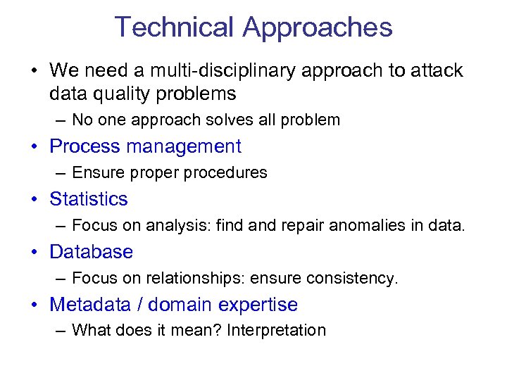Technical Approaches • We need a multi-disciplinary approach to attack data quality problems – No one approach solves all problem • Process management – Ensure proper procedures • Statistics – Focus on analysis: find and repair anomalies in data. • Database – Focus on relationships: ensure consistency. • Metadata / domain expertise – What does it mean? Interpretation

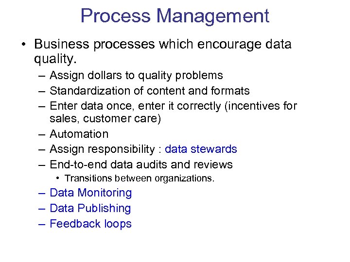Process Management • Business processes which encourage data quality. – Assign dollars to quality problems – Standardization of content and formats – Enter data once, enter it correctly (incentives for sales, customer care) – Automation – Assign responsibility : data stewards – End-to-end data audits and reviews • Transitions between organizations. – Data Monitoring – Data Publishing – Feedback loops

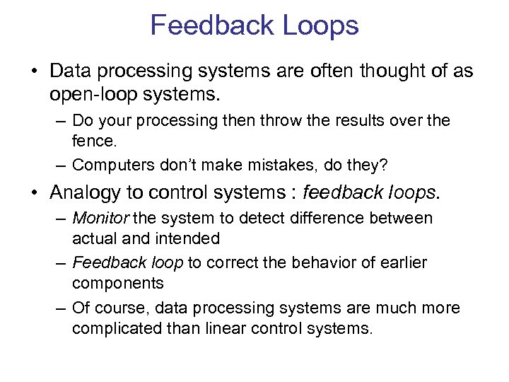Feedback Loops • Data processing systems are often thought of as open-loop systems. – Do your processing then throw the results over the fence. – Computers don’t make mistakes, do they? • Analogy to control systems : feedback loops. – Monitor the system to detect difference between actual and intended – Feedback loop to correct the behavior of earlier components – Of course, data processing systems are much more complicated than linear control systems.

Example • Sales, provisioning, and billing for telecommunications service – Many stages involving handoffs between organizations and databases – Simplified picture • Transition between organizational boundaries is a common cause of problems. • Natural feedback loops – Customer complains if the bill is to high • Missing feedback loops – No complaints if we undercharge.

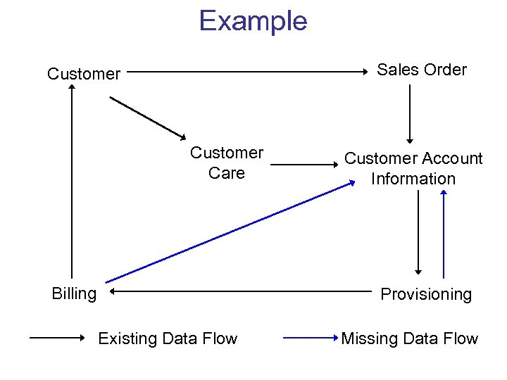Example Sales Order Customer Care Billing Customer Account Information Provisioning Existing Data Flow Missing Data Flow

Monitoring • Use data monitoring to add missing feedback loops. • Methods: – Data tracking / auditing • Follow a sample of transactions through the workflow. • Build secondary processing system to detect possible problems. – Reconciliation of incrementally updated databases with original sources. – Mandated consistency with a Database of Record (DBOR). – Feedback loop sync-up – Data Publishing

Data Publishing • Make the contents of a database available in a readily accessible and digestible way – Web interface (universal client). – Data Squashing : Publish aggregates, cubes, samples, parametric representations. – Publish the metadata. • Close feedback loops by getting a lot of people to look at the data. • Surprisingly difficult sometimes. – Organizational boundaries, loss of control interpreted as loss of power, desire to hide problems.

Statistical Approaches • No explicit DQ methods – Traditional statistical data collected from carefully designed experiments, often tied to analysis – But, there are methods for finding anomalies and repairing data. – Existing methods can be adapted for DQ purposes. • Four broad categories can be adapted for DQ – Missing, incomplete, ambiguous or damaged data e. g truncated, censored – Suspicious or abnormal data e. g. outliers – Testing for departure from models – Goodness-of-fit

Missing Data • Missing data - values, attributes, entire records, entire sections • Missing values and defaults are indistinguishable • Truncation/censoring - not aware, mechanisms not known • Problem: Misleading results, bias.

Detecting Missing Data • Overtly missing data – Match data specifications against data - are all the attributes present? – Scan individual records - are there gaps? – Rough checks : number of files, file sizes, number of records, number of duplicates – Compare estimates (averages, frequencies, medians) with “expected” values and bounds; check at various levels of granularity since aggregates can be misleading.

Missing data detection (cont. ) • Hidden damage to data – Values are truncated or censored - check for spikes and dips in distributions and histograms – Missing values and defaults are indistinguishable - too many missing values? metadata or domain expertise can help – Errors of omission e. g. all calls from a particular area are missing - check if data are missing randomly or are localized in some way

Imputing Values to Missing Data • In federated data, between 30%-70% of the data points will have at least one missing attribute - data wastage if we ignore all records with a missing value • Remaining data is seriously biased • Lack of confidence in results • Understanding pattern of missing data unearths data integrity issues

Missing Value Imputation - 1 • Standalone imputation – Mean, median, other point estimates – Assume: Distribution of the missing values is the same as the non-missing values. – Does not take into account inter-relationships – Introduces bias – Convenient, easy to implement

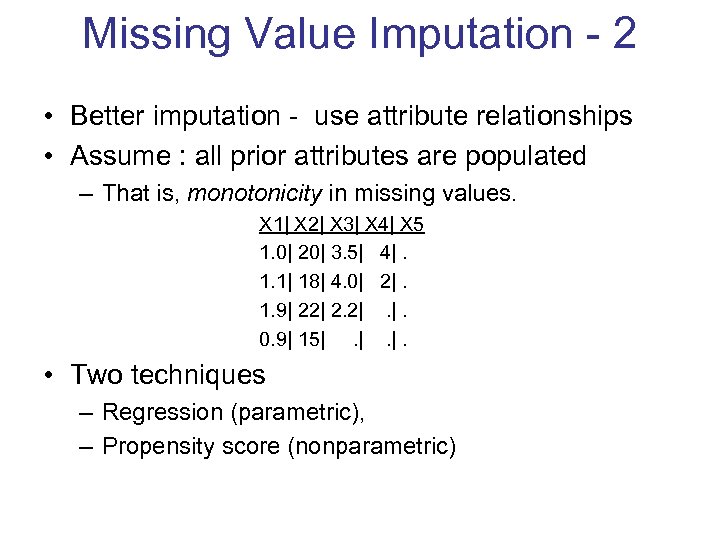Missing Value Imputation - 2 • Better imputation - use attribute relationships • Assume : all prior attributes are populated – That is, monotonicity in missing values. X 1| X 2| X 3| X 4| X 5 1. 0| 20| 3. 5| 4|. 1. 1| 18| 4. 0| 2|. 1. 9| 22| 2. 2|. |. 0. 9| 15|. |. |. • Two techniques – Regression (parametric), – Propensity score (nonparametric)

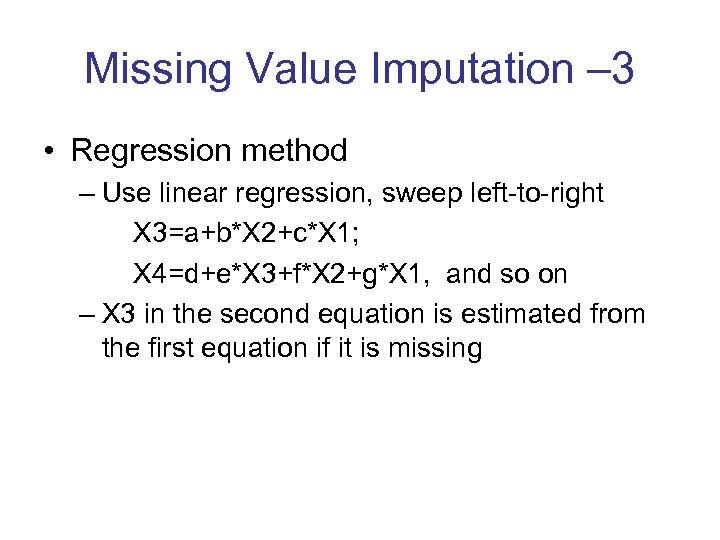Missing Value Imputation – 3 • Regression method – Use linear regression, sweep left-to-right X 3=a+b*X 2+c*X 1; X 4=d+e*X 3+f*X 2+g*X 1, and so on – X 3 in the second equation is estimated from the first equation if it is missing

Missing Value Imputation - 3 • Propensity Scores (nonparametric) – Let Yj=1 if Xj is missing, 0 otherwise – Estimate P(Yj =1) based on X 1 through X(j-1) using logistic regression – Group by propensity score P(Yj =1) – Within each group, estimate missing Xjs from known Xjs using approximate Bayesian bootstrap. – Repeat until all attributes are populated.

Missing Value Imputation - 4 • Arbitrary missing pattern – Markov Chain Monte Carlo (MCMC) – Assume data is multivariate Normal, with parameter Q – (1) Simulate missing X, given Q estimated from observed X ; (2) Re-compute Q using filled in X – Repeat until stable. – Expensive: Used most often to induce monotonicity • Note that imputed values are useful in aggregates but can’t be trusted individually

Censoring and Truncation • Well studied in Biostatistics, relevant to time dependent data e. g. duration • Censored - Measurement is bounded but not precise e. g. Call duration > 20 are recorded as 20 • Truncated - Data point dropped if it exceeds or falls below a certain bound e. g. customers with less than 2 minutes of calling per month

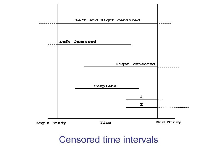Censored time intervals

Censoring/Truncation (cont. ) • If censoring/truncation mechanism not known, analysis can be inaccurate and biased. • But if you know the mechanism, you can mitigate the bias from the analysis. • Metadata should record the existence as well as the nature of censoring/truncation

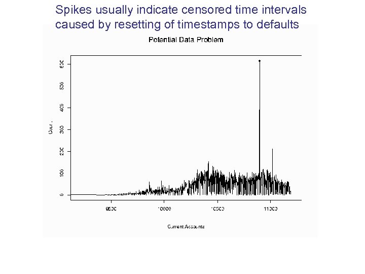Spikes usually indicate censored time intervals caused by resetting of timestamps to defaults

Suspicious Data • Consider the data points 3, 4, 7, 4, 8, 3, 9, 5, 7, 6, 92 • “ 92” is suspicious - an outlier • Outliers are potentially legitimate • Often, they are data or model glitches • Or, they could be a data miner’s dream, e. g. highly profitable customers

Outliers • Outlier – “departure from the expected” • Types of outliers – defining “expected” • Many approaches – Error bounds, tolerance limits – control charts – Model based – regression depth, analysis of residuals – Geometric – Distributional – Time Series outliers

Control Charts • Quality control of production lots • Typically univariate: X-Bar, R, CUSUM • Distributional assumptions for charts not based on means e. g. R–charts • Main steps (based on statistical inference) – Define “expected” and “departure” e. g. Mean and standard error based on sampling distribution of sample mean (aggregate); – Compute aggregate each sample – Plot aggregates vs expected and error bounds – “Out of Control” if aggregates fall outside bounds

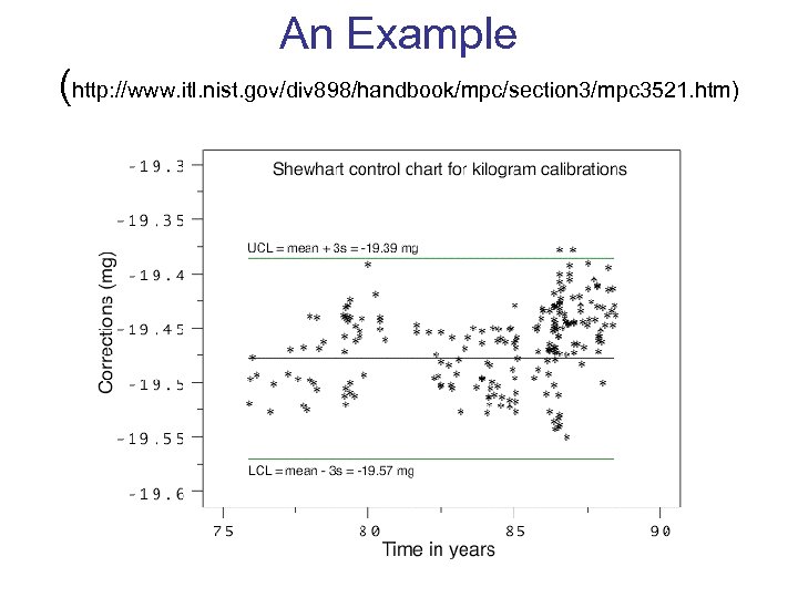An Example (http: //www. itl. nist. gov/div 898/handbook/mpc/section 3/mpc 3521. htm)

Multivariate Control Charts - 1 • Bivariate charts: – based on bivariate Normal assumptions – component-wise limits lead to Type I, II errors • Depth based control charts (nonparametric): – map n-dimensional data to one dimension using depth e. g. Mahalanobis – Build control charts for depth – Compare against benchmark using depth e. g. Q-Q plots of depth of each data set

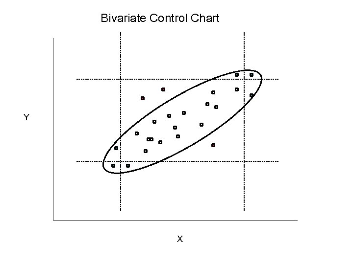Bivariate Control Chart Y X

Multivariate Control Charts - 2 • Multiscale process control with wavelets: – Detects abnormalities at multiple scales as large wavelet coefficients. – Useful for data with heteroscedasticity – Applied in chemical process control

Model Fitting and Outliers • Models summarize general trends in data – more complex than simple aggregates – e. g. linear regression, logistic regression focus on attribute relationships • Data points that do not conform to well fitting models are potential outliers • Goodness of fit tests (DQ for analysis/mining) – check suitableness of model to data – verify validity of assumptions – data rich enough to answer analysis/business question?

Set Comparison and Outlier Detection • “Model” consists of partition based summaries • Perform nonparametric statistical tests for a rapid section-wise comparison of two or more massive data sets • If there exists a baseline “good’’ data set, this technique can detect potentially corrupt sections in the test data set

Goodness of Fit - 1 • Chi-square test – Are the attributes independent? – Does the observed (discrete) distribution match the assumed distribution? • • Tests for Normality Q-Q plots (visual) Kolmogorov-Smirnov test Kullback-Liebler divergence

Goodness of Fit - 2 • Analysis of residuals – Departure of individual points from model – Patterns in residuals reveal inadequacies of model or violations of assumptions – Reveals bias (data are non-linear) and peculiarities in data (variance of one attribute is a function of other attributes) – Residual plots

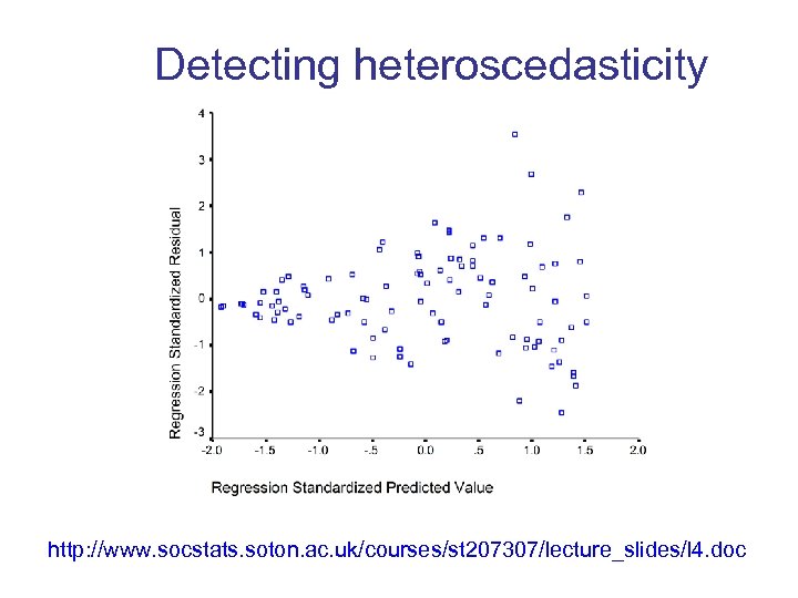Detecting heteroscedasticity http: //www. socstats. soton. ac. uk/courses/st 207307/lecture_slides/l 4. doc

Goodness of Fit -3 • Regression depth – measures the “outlyingness” of a model, not an individual data point – indicates how well a regression plane represents the data – If a regression plane needs to pass through many points to rotate to the vertical (non-fit) position, it has high regression depth

Geometric Outliers • Define outliers as those points at the periphery of the data set. • Peeling : define layers of increasing depth, outer layers contain the outlying points – Convex Hull: peel off successive convex hull points. – Depth Contours: layers are the data depth layers. • Efficient algorithms for 2 -D, 3 -D. • Computational complexity increases rapidly with dimension. – Ω(Nceil(d/2)) complexity for N points, d dimensions

Distributional Outliers • For each point, compute the maximum distance to its k nearest neighbors. – DB(p, D)-outlier : at least fraction p of the points in the database lie at distance greater than D. • Fast algorithms – One is O(d. N 2), one is O(cd+N) • Local Outliers : adjust definition of outlier based on density of nearest data clusters.

Time Series Outliers • Data is a time series of measurements of a large collection of entities (e. g. customer usage). • Vector of measurements define a trajectory for an entity. • A trajectory can be glitched, and it can make radical but valid changes. • Approach: develop models based on entity’s past behavior (within) and all entity behavior (relative). • Find potential glitches: – Common glitch trajectories – Deviations from within and relative behavior.