Data Preparation for Knowledge Discovery Outline Data

Data Preparation for Knowledge Discovery

Outline: Data Preparation § Data Understanding § Data Cleaning § Metadata § Missing Values § Unified Date Format § Nominal to Numeric § Discretization § Field Selection and “False Predictors” § Unbalanced Target Distribution 2

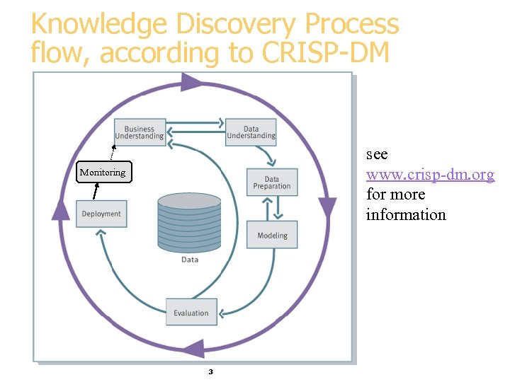Knowledge Discovery Process flow, according to CRISP-DM see www. crisp-dm. org for more information Monitoring 3

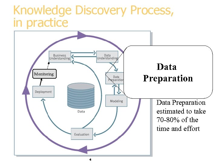Knowledge Discovery Process, in practice Data Preparation Monitoring Data Preparation estimated to take 70 -80% of the time and effort 4

Data Understanding: Relevance § What data is available for the task? § Is this data relevant? § Is additional relevant data available? § How much historical data is available? § Who is the data expert ? 5

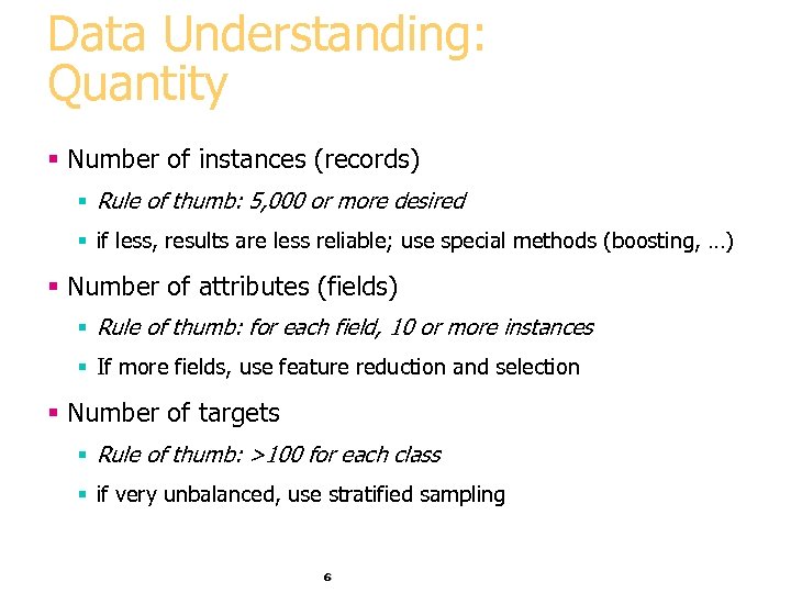Data Understanding: Quantity § Number of instances (records) § Rule of thumb: 5, 000 or more desired § if less, results are less reliable; use special methods (boosting, …) § Number of attributes (fields) § Rule of thumb: for each field, 10 or more instances § If more fields, use feature reduction and selection § Number of targets § Rule of thumb: >100 for each class § if very unbalanced, use stratified sampling 6

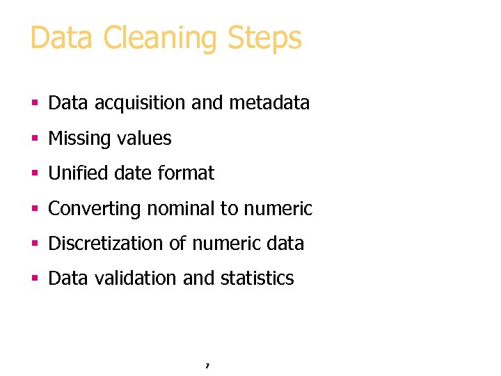Data Cleaning Steps § Data acquisition and metadata § Missing values § Unified date format § Converting nominal to numeric § Discretization of numeric data § Data validation and statistics 7

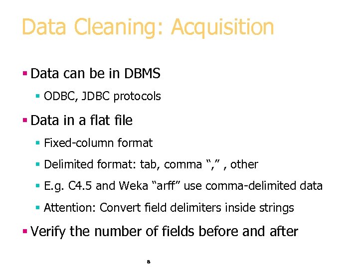Data Cleaning: Acquisition § Data can be in DBMS § ODBC, JDBC protocols § Data in a flat file § Fixed-column format § Delimited format: tab, comma “, ” , other § E. g. C 4. 5 and Weka “arff” use comma-delimited data § Attention: Convert field delimiters inside strings § Verify the number of fields before and after 8

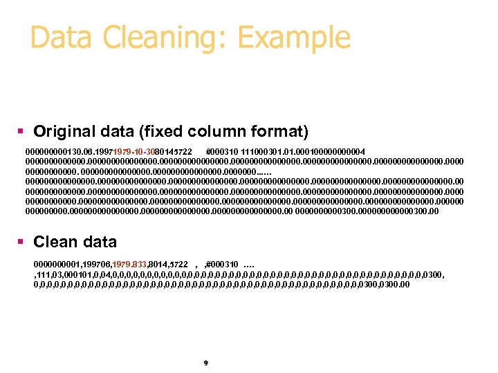Data Cleaning: Example § Original data (fixed column format) 00000130. 06. 19971979 -10 -3080145722 #000310 111000301. 0001000004 000000000000000. 0000000. . . … 000000000000000. 00 00000000000000000000000000. 00000000. 00 0000000000300. 00 § Clean data 000001, 199706, 1979. 833, 8014, 5722 , , #000310 …. , 111, 03, 000101, 0, 04, 0, 0, 0, 0, 0, 0, 0, 0, 0, 0, 0, 0300, 0, 0, 0, 0, 0, 0, 0, 0, 0, 0, 0, 0300, 0300. 00 9

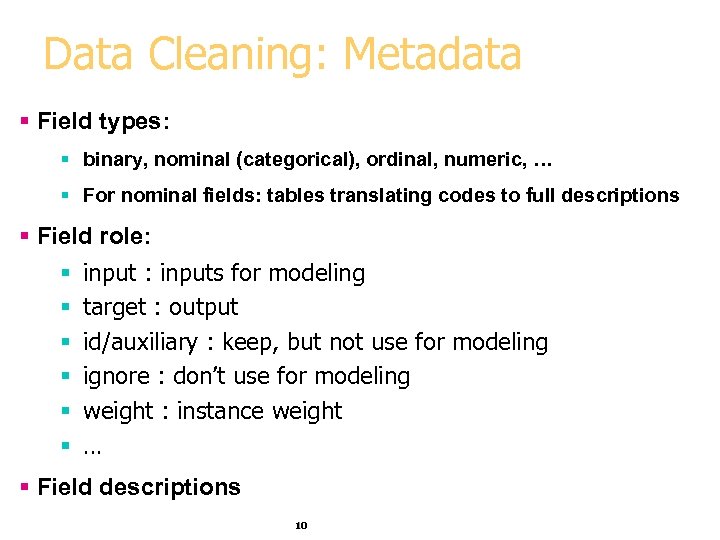Data Cleaning: Metadata § Field types: § binary, nominal (categorical), ordinal, numeric, … § For nominal fields: tables translating codes to full descriptions § Field role: § input : inputs for modeling § target : output § id/auxiliary : keep, but not use for modeling § ignore : don’t use for modeling § weight : instance weight § … § Field descriptions 10

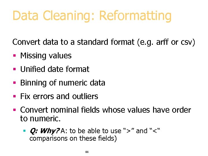Data Cleaning: Reformatting Convert data to a standard format (e. g. arff or csv) § Missing values § Unified date format § Binning of numeric data § Fix errors and outliers § Convert nominal fields whose values have order to numeric. § Q: Why? A: to be able to use “>” and “<“ comparisons on these fields) 11

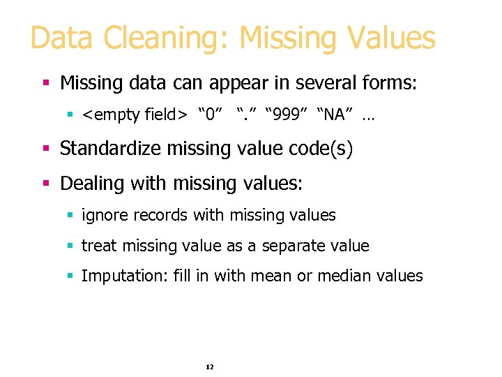Data Cleaning: Missing Values § Missing data can appear in several forms: § “ 0” “. ” “ 999” “NA” … § Standardize missing value code(s) § Dealing with missing values: § ignore records with missing values § treat missing value as a separate value § Imputation: fill in with mean or median values 12

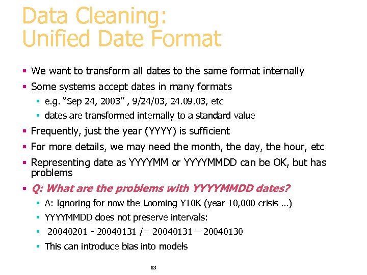Data Cleaning: Unified Date Format § We want to transform all dates to the same format internally § Some systems accept dates in many formats § e. g. “Sep 24, 2003” , 9/24/03, 24. 09. 03, etc § dates are transformed internally to a standard value § Frequently, just the year (YYYY) is sufficient § For more details, we may need the month, the day, the hour, etc § Representing date as YYYYMM or YYYYMMDD can be OK, but has problems § Q: What are the problems with YYYYMMDD dates? § A: Ignoring for now the Looming Y 10 K (year 10, 000 crisis …) § YYYYMMDD does not preserve intervals: § 20040201 - 20040131 /= 20040131 – 20040130 § This can introduce bias into models 13

Unified Date Format Options § To preserve intervals, we can use § Unix system date: Number of seconds since 1970 § Number of days since Jan 1, 1960 (SAS) § Problem: § values are non-obvious § don’t help intuition and knowledge discovery § harder to verify, easier to make an error 14

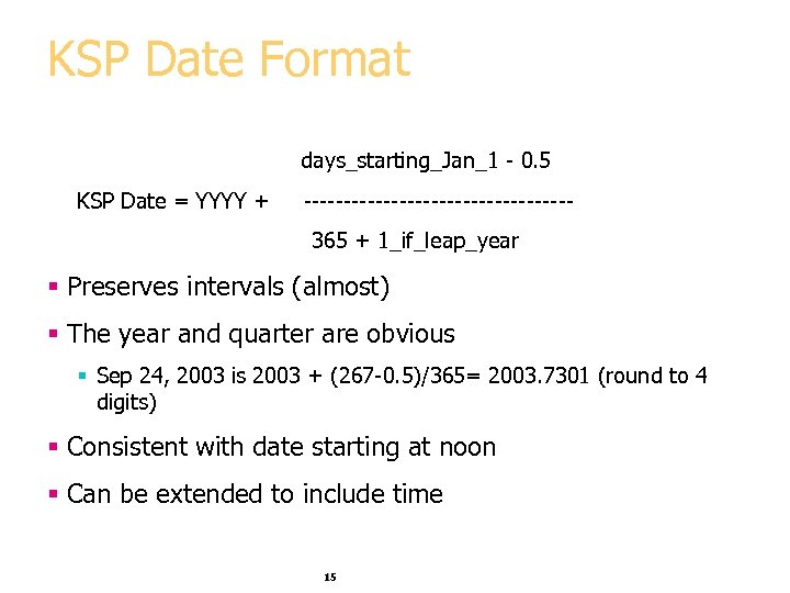KSP Date Format days_starting_Jan_1 - 0. 5 KSP Date = YYYY + -----------------365 + 1_if_leap_year § Preserves intervals (almost) § The year and quarter are obvious § Sep 24, 2003 is 2003 + (267 -0. 5)/365= 2003. 7301 (round to 4 digits) § Consistent with date starting at noon § Can be extended to include time 15

Y 2 K issues: 2 digit Year § 2 -digit year in old data – legacy of Y 2 K § E. g. Q: Year 02 – is it 1902 or 2002 ? § A: Depends on context (e. g. child birthday or year of house construction) § Typical approach: CUTOFF year, e. g. 30 § if YY < CUTOFF , then 20 YY, else 19 YY 16

Conversion: Nominal to Numeric § Some tools can deal with nominal values internally § Other methods (neural nets, regression, nearest neighbor) require only numeric inputs § To use nominal fields in such methods need to convert them to a numeric value § Q: Why not ignore nominal fields altogether? § A: They may contain valuable information § Different strategies for binary, ordered, multivalued nominal fields 17

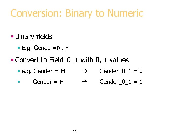Conversion: Binary to Numeric § Binary fields § E. g. Gender=M, F § Convert to Field_0_1 with 0, 1 values § e. g. Gender = M § Gender = F 18 Gender_0_1 = 0 Gender_0_1 = 1

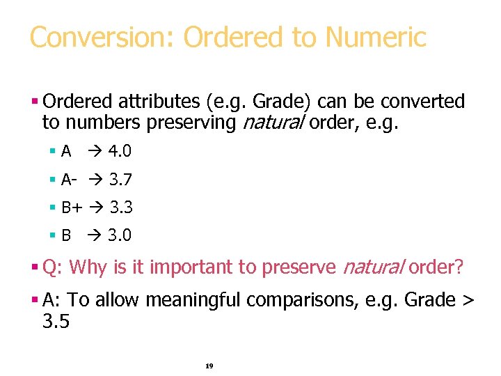Conversion: Ordered to Numeric § Ordered attributes (e. g. Grade) can be converted to numbers preserving natural order, e. g. § A 4. 0 § A- 3. 7 § B+ 3. 3 § B 3. 0 § Q: Why is it important to preserve natural order? § A: To allow meaningful comparisons, e. g. Grade > 3. 5 19

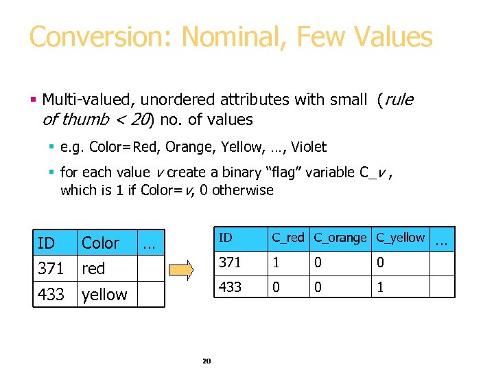Conversion: Nominal, Few Values § Multi-valued, unordered attributes with small (rule of thumb < 20) no. of values § e. g. Color=Red, Orange, Yellow, …, Violet § for each value v create a binary “flag” variable C_v , which is 1 if Color=v, 0 otherwise ID C_red C_orange C_yellow red 371 1 0 0 yellow 433 0 0 1 ID Color 371 433 … 20 …

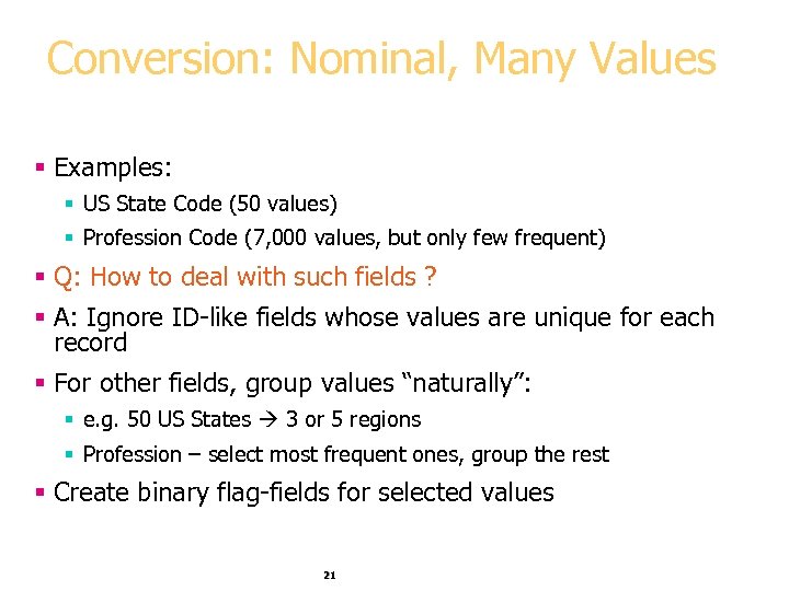Conversion: Nominal, Many Values § Examples: § US State Code (50 values) § Profession Code (7, 000 values, but only few frequent) § Q: How to deal with such fields ? § A: Ignore ID-like fields whose values are unique for each record § For other fields, group values “naturally”: § e. g. 50 US States 3 or 5 regions § Profession – select most frequent ones, group the rest § Create binary flag-fields for selected values 21

Data Cleaning: Discretization § Some methods require discrete values, e. g. most versions of Naïve Bayes, CHAID § Discretization is very useful for generating a summary of data § Also called “binning” 22

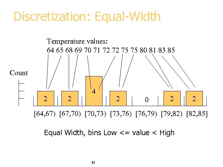Discretization: Equal-Width Temperature values: 64 65 68 69 70 71 72 72 75 75 80 81 83 85 Count 2 2 4 2 0 2 2 [64, 67) [67, 70) [70, 73) [73, 76) [76, 79) [79, 82) [82, 85] Equal Width, bins Low <= value < High 23

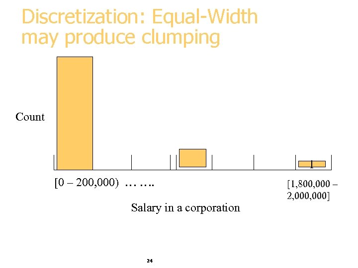Discretization: Equal-Width may produce clumping Count 1 [0 – 200, 000) … …. Salary in a corporation 24 [1, 800, 000 – 2, 000]

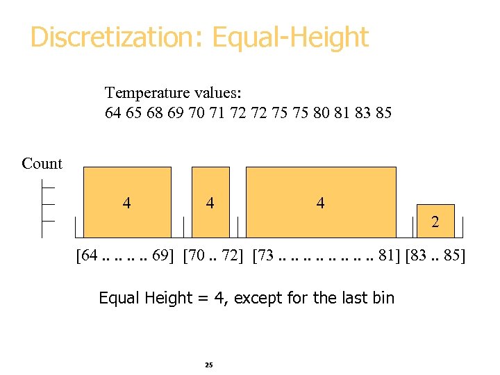Discretization: Equal-Height Temperature values: 64 65 68 69 70 71 72 72 75 75 80 81 83 85 Count 4 4 4 2 [64. . . . 69] [70. . 72] [73. . . . 81] [83. . 85] Equal Height = 4, except for the last bin 25

Discretization: Equal-height advantages § Generally preferred because avoids clumping § In practice, “almost-equal” height binning is used which avoids clumping and gives more intuitive breakpoints § Additional considerations: § don’t split frequent values across bins § create separate bins for special values (e. g. 0) § readable breakpoints (e. g. round breakpoints) 26

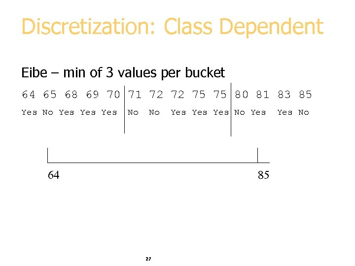Discretization: Class Dependent Eibe – min of 3 values per bucket 64 65 68 69 70 71 72 72 75 75 80 81 83 85 Yes No Yes Yes No No 64 Yes Yes No Yes 85 27 Yes No

Discretization considerations § Equal Width is simplest, good for many classes § can fail miserably for unequal distributions § Equal Height gives better results § Class-dependent can be better for classification § Note: decision trees build discretization on the fly § Naïve Bayes requires initial discretization § Many other methods exist … 28

Outliers and Errors § Outliers are values thought to be out of range. § Approaches: § do nothing § enforce upper and lower bounds § let binning handle the problem 29

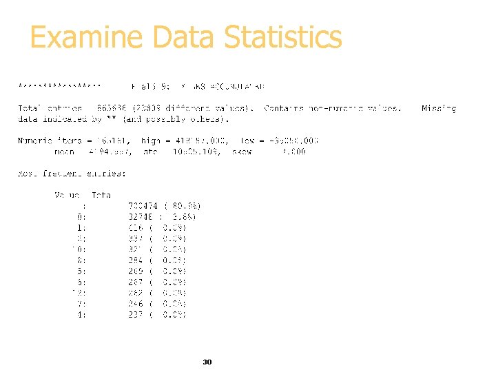Examine Data Statistics 30

Data Cleaning: Field Selection First: Remove fields with no or little variability § Examine the number of distinct field values § Rule of thumb: remove a field where almost all values are the same (e. g. null), except possibly in minp % or less of all records. § minp could be 0. 5% or more generally less than 5% of the number of targets of the smallest class 31

False Predictors or Information “Leakers” § False predictors are fields correlated to target behavior, which describe events that happen at the same time or after the target behavior § If databases don’t have the event dates, a false predictor will appear as a good predictor § Example: Service cancellation date is a leaker when predicting attriters. § Q: Give another example of a false predictor § A: e. g. student final grade, for the task of predicting whether the student passed the course 32

False Predictors: Find “suspects” § Build an initial decision-tree model § Consider very strongly predictive fields as “suspects” § strongly predictive – if a field by itself provides close to 100% accuracy, at the top or a branch below § Verify “suspects” using domain knowledge or with a domain expert § Remove false predictors and build an initial model 33

(Almost) Automated False Predictor Detection § For each field § Build 1 -field decision trees for each field § (or compute correlation with the target field) § Rank all suspects by 1 -field prediction accuracy (or correlation) § Remove suspects whose accuracy is close to 100% (Note: the threshold is domain dependent) § Verify top “suspects” with domain expert 34

Selecting Most Relevant Fields § If there are too many fields, select a subset that is most relevant. § Can select top N fields using 1 -field predictive accuracy as computed earlier. § What is good N? § Rule of thumb -- keep top 50 fields 35

Field Reduction Improves Classification § most learning algorithms look for non-linear combinations of fields -- can easily find many spurious combinations given small # of records and large # of fields § Classification accuracy improves if we first reduce number of fields § Multi-class heuristic: select equal # of fields from each class 36

Derived Variables § Better to have a fair modeling method and good variables, than to have the best modeling method and poor variables. § Insurance Example: People are eligible for pension withdrawal at age 59 ½. Create it as a separate Boolean variable! § *Advanced methods exists for automatically examining variable combinations, but it is very computationally expensive! 37

Unbalanced Target Distribution § Sometimes, classes have very unequal frequency § Attrition prediction: 97% stay, 3% attrite (in a month) § medical diagnosis: 90% healthy, 10% disease § e. Commerce: 99% don’t buy, 1% buy § Security: >99. 99% of Americans are not terrorists § Similar situation with multiple classes § Majority classifier can be 97% correct, but useless 38

Handling Unbalanced Data § With two classes: let positive targets be a minority § Separate raw held-aside set (e. g. 30% of data) and raw train § put aside raw held-aside and don’t use it till the final model § Select remaining positive targets (e. g. 70% of all targets) from raw train § Join with equal number of negative targets from raw train, and randomly sort it. § Separate randomized balanced set into balanced train and balanced test 39

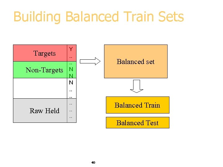Building Balanced Train Sets Targets Non-Targets Raw Held Y. . N N N. . Balanced set Balanced Train Balanced Test 40

Learning with Unbalanced Data § Build models on balanced train/test sets § Estimate the final results (lift curve) on the raw held set § Can generalize “balancing” to multiple classes § stratified sampling § Ensure that each class is represented with approximately equal proportions in train and test 41

Data Preparation Key Ideas § Use meta-data § Inspect data for anomalies and errors § Eliminate “false positives” § Develop small, reusable software components § Plan for verification - verify the results after each step 42

Summary Good data preparation is key to producing valid and reliable models 43